A joke in approximating numbers raised to irrational powers
How it started
This story began, unexpectedly, on Facebook in a math-focused group. A teacher asked the group to determine the value of: \(\lfloor 3^{\sqrt{3}}\rfloor\) without using a calculator.
Naturally, the challenge was to prove whether \(\lfloor 3^{\sqrt{3}}\rfloor=6\) or \(\lfloor 3^{\sqrt{3}}\rfloor=7\) (my intuition leaned toward 7).
Eventually, the most convincing solution, proposed by Mihai Cris, was accepted by the group:
And on the other end:
Since \(\sqrt{3}\approx 1.73 \Rightarrow \lfloor 3^{\sqrt{3}}\rfloor=6\).
Later edit:
After sharing the post on reddit, user /u/JiminP proposed an alternative method:
Simultaneously:
Which method is better? That’s left to the reader.
The new problem
That problem was charming—but it sparked a bigger question:
Could we approximate small numbers raised to irrational powers without using calculators, logs, or radicals—just addition and multiplication?
This was more of a joke than a serious challenge, so here’s my final formula (if you don’t want to read the rest):
(… as long as \(\frac{1}{2} < \ln a * \sqrt{c} < 3\))
The first attempt
The Logarithmic and the Exponential functions came to the rescue.
- We start by writing \(3^{\sqrt{3}}=(e^{\ln 3})^{\sqrt{3}}=e^{\sqrt{3}\ln 3}\). We know this is true because \(3=e^{\ln 3}=3^{\ln e}=3\).
- We then use the Taylor Series expansion of \(e^x=1+\frac{x^1}{1!}+\frac{x^2}{2!}+\frac{x^3}{3!}+\frac{x^4}{4!}+\dots\) .
- Therefore, approximating \(3^{\sqrt{3}}\) becomes a matter of computing: \(1+\frac{(\sqrt{3}\ln 3)^1}{1!}+\frac{(\sqrt{3}\ln 3)^2}{2!}+\frac{(\sqrt{3}\ln 3)^3}{3!}+\frac{(\sqrt{3}\ln 3)^4}{4!}+\dots\).
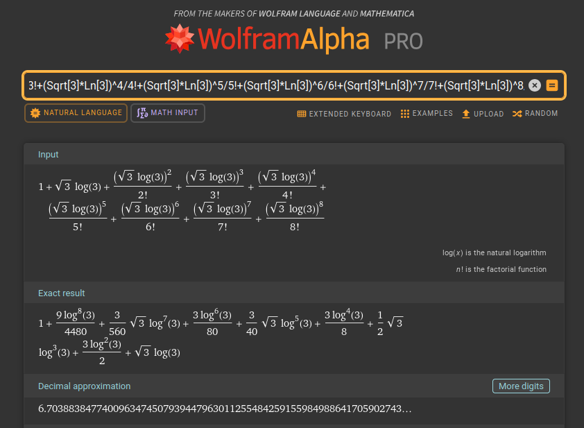
To get even closer to the actual result, I computed the first 8 terms of the series expansion (and no, it wasn’t by hand, as I’ve used WolframAlpha do it for me):
1+Sqrt[3]*Ln[3]+(Sqrt[3]*Ln[3])^2/2!+(Sqrt[3]*Ln[3])^3/3!+(Sqrt[3]*Ln[3])^4/4!+(Sqrt[3]*Ln[3])^5/5!+(Sqrt[3]*Ln[3])^6/6!+(Sqrt[3]*Ln[3])^7/7!+(Sqrt[3]*Ln[3])^8/8!
The eureka!
At this point I had a few flashbacks from my school days, and two ideas resurfaced.
Firstly, there was something called Small Angle Approximations, that happen when the angle is, as you would expect, (very) very small:
So I’ve wondered if there isn’t something similar for \(e^x, \ln x\) and \(\sqrt{x}\), anything that works for small numbers.
Secondly, I remember watching a few months ago a video from Michael Penn, about something called Padé Approximations: Pade Approximation – unfortunately missed in most Caclulus courses. It was a subject worth exploring.
Pade approximations are “smooth”
So, without going into too much details, a Padé approximation is a rational function (the ratio of two polynomials) used to represent a given function. The smart idea behind this technique is to distribute the control points of a polynomial between the denominator and the numerator of the rational function.
A Padé approximation of order [m/n] for a function \(f(x)\) is expressed as:
Compared to Taylor Series, Padé seem to handle exponential behaviors and discontinuities better, plus in a lot of cases it converges faster.
Needless to say, I was curious how well those approximations actually work, so I’ve computed the Padé aproximation of order [1/1], \(P_{[1/1]}(x)\) for \(e^x\). (For in depth tutorial follow the Professor’s Penn tutorial, linked above).
To find \(a_0, a_1, b_1\) we need to solve the following system of equations:
After solving this, we will get \(P_{[1/1]}=\frac{2+x}{2-x}\).
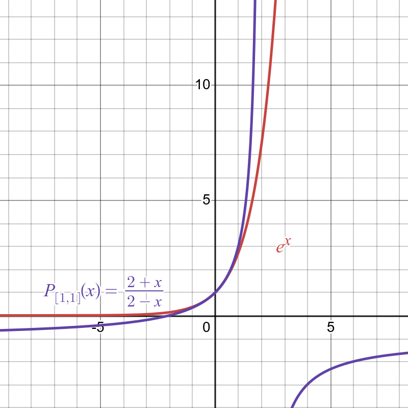
We can already see that the \(P_{[1/1]}\) follows nicely \(e^x\) for the numbers around \(0\).
\(P_{[2/2]}=\frac{x^2+6x+12}{x^2-6x+12}\) is even better at approximating \(e^x\), at least up to a certain point.
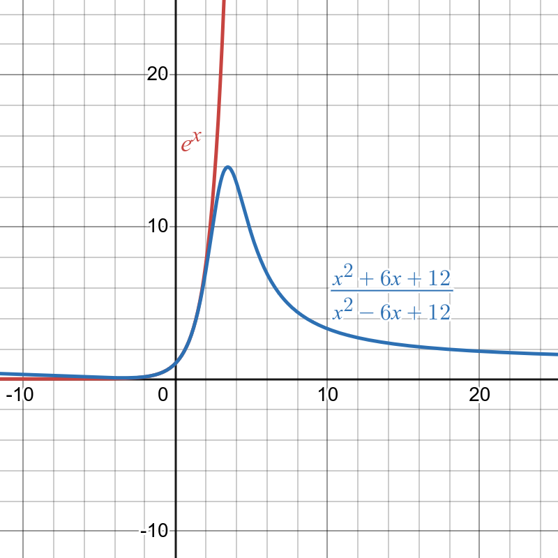
So, in a way, \(e^x \approx \frac{x^2+6x+12}{x^2-6x+12}\) is true for small numbers, just like \(\sin(x) \approx x\) is true for small angles.
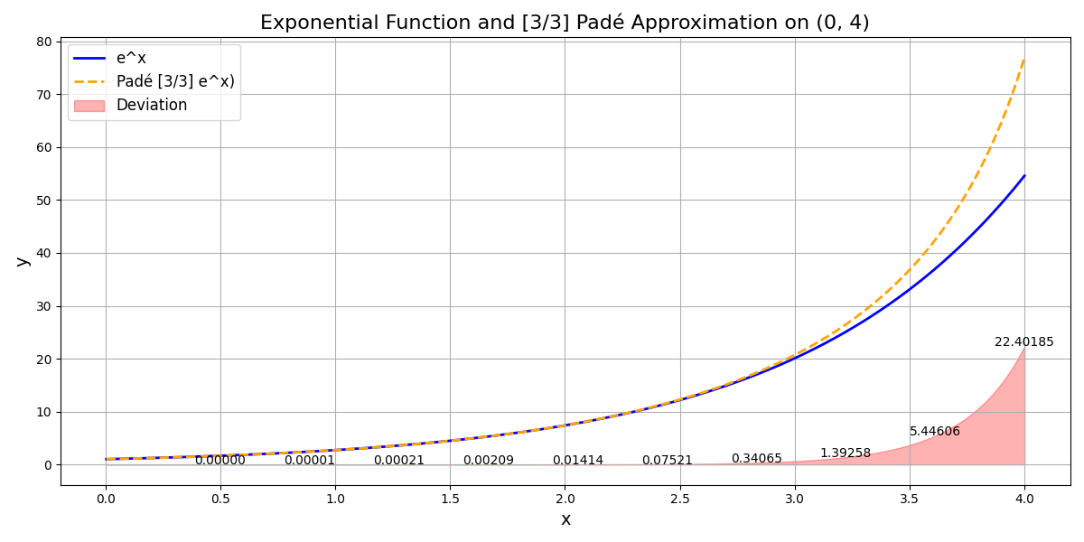
Or, even better, \(e^x \approx \frac{-120-60x-12x^{2}-x^{3}}{-120+60x-12x^{2}+x^{3}}\) is true for small small numbers, just like \(\sin(x) \approx x\) is true for small angles.
And it’s get better, for the \(\ln x\) function the equivalent [2/2] Padé approximation is: \(\frac{3(x-1)(x+1)}{x^{2}+4x+1}\). Notice how the approximation is bad if \(x < 0.5\). For this we should find a better function.
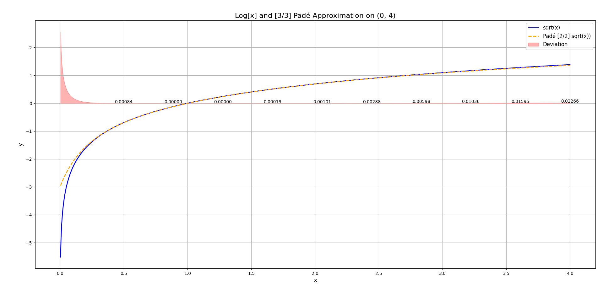
Note: While the exponential function is approximated around \(x=0\) (a Maclaurin series), the approximations for \(\ln (x)\) and \(x\) are centered at \(x=1\). This is because \(\ln (0)\) is undefined, and we want our rational functions to be most accurate in the range of the small positive integers we are testing.
And for \(\sqrt{x}\) the [2/2] approximation will be \(\frac{5x^{2}+10x+1}{x^{2}+10x+5}\).
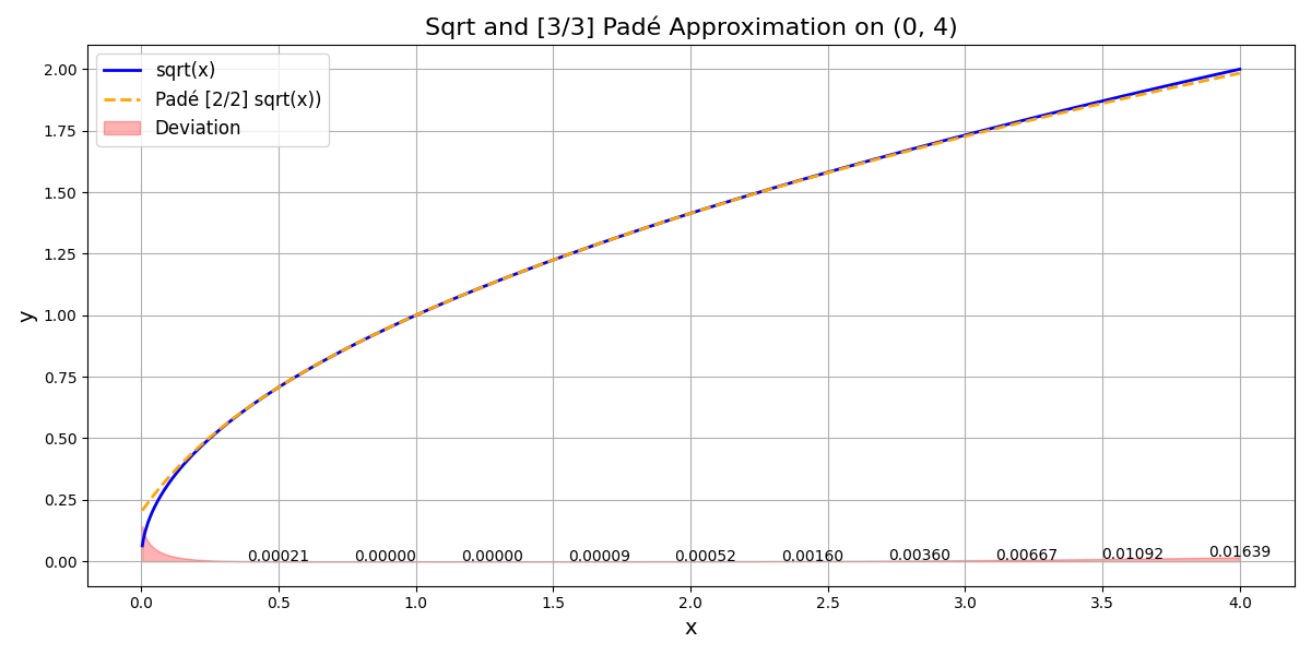
The “monster” function
Putting all together.
- To compute \(e^x\) for \(x \in (0,4)\), we use: \(\frac{-120-60x-12x^{2}-x^{3}}{-120+60x-12x^{2}+x^{3}}\).
- To compute \(\ln x\) for \(x \in (0.5, 4)\) we use: \(\frac{3(x-1)(x+1)}{x^{2}+4x+1}\).
- To compute \(\sqrt{x}\) for \(x \in (0, 4)\) we use: \(\frac{5x^{2}+10x+1}{x^{2}+10x+5}\).
So for “small numbers” we can approximate \(a^b\) using the following expression:
Or we can compute:
Testing the “monster” function
Now, to test our marvelous approximation, let’s compute \(2^{\sqrt{2}}\):
- We start approximating the logarithm: \(\ln 2=\frac{3(2-1)(2+1)}{2^2+8+1}=\frac{3*1*3}{4+8+1}=\frac{9}{13} \approx 0.69\).
- We continue approximating the radical: \(\sqrt{2}=\frac{5*2^2+20+1}{4+20+5}=\frac{20+20+1}{29}=\frac{41}{29} \approx 1.41\)
- We compute the product: \(0.69*1.41 \approx 0.97\).
- We actually compute the power: \(2^{\sqrt{2}}=e^{\sqrt{2}\ln 2} \approx e^{0.97}=\frac{-120-60*(0.97)-12*(0.97)^{2}-(0.97)^{3}}{-120+60*(0.97)-12*(0.97)^{2}+(0.97)^{3}} \approx 2.6612\)
The actual result should’ve been: \(2.6651\). Not bad.
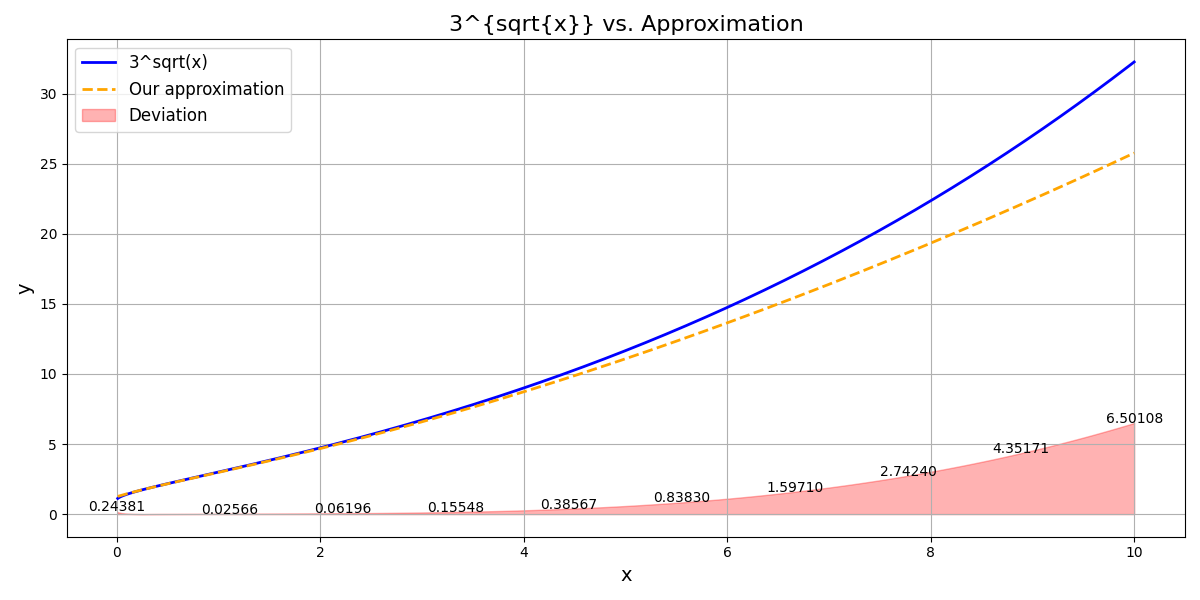
Computing \(3^{\sqrt{3}}\) with our function yields: \(6.58\) instead of \(6.70\). Not terrible.
The deviation for \(0.1^{\sqrt{x}}\), \(2^{\sqrt{x}}\) and \(3^{\sqrt{x}}\)
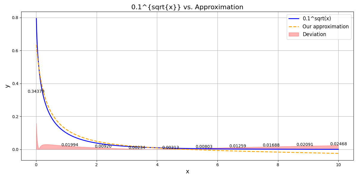
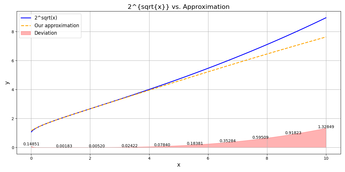
Final thoughts
-
The monster function is clearly impractical—especially in the era of logic gates and floating-point math. But that wasn’t the point.
-
This post was just a fun excuse to explore Padé Approximations firsthand.
-
I briefly considered extending this technique to Fourier series. While some research exists on “rationalizing” Fourier series to reduce Gibbs phenomena, Padé approximations lose periodicity, so it’s a tricky compromise.

Comments