
From the Circle to Epicycles (Part 1) - An animated introduction to Fourier Series
This article will be part of an extensive series in which I plan to explore various aspects of Fourier Mathematics. I will take notes, create some visuals (a good pretext to learn more about graphics), and hope that it will be helpful to anyone looking for a clear, visual introduction to these concepts.
The article has yet to be thoroughly reviewed by anyone other than me, so I put it online, hoping to get some feedback before bringing it to a final state.
Table of contents
In this series, we will start with a brief recap of some of the math concepts related to the circle, including trigonometric functions like sine and cosine. We’ll also discuss Euler’s identity, introduce the concept of a sinusoid (and complex sinusoid), and finally, we’ll introduce the concept of Fourier Series.
The animations used in this series are original, although I drew inspiration from some existing materials found on the web. Please keep in mind that this is not a comprehensive course on the topic, so if you’re really interested in learning more, I recommend taking a full course on the subject.
- Table of contents
- The Circle
- The number \(\pi\)
- Radians
- The sine and the cosine
- The \(\cos\) leads the \(\sin\)
- The parity of \(\cos\) and \(\sin\)
- Complex Numbers and the Unit Circle
- Multiplying with \(i\) means a rotation with \(\frac{\pi}{2}\)
- Euler’s identity
- Euler’s formula, the connection between \(e\), \(\\pi\) and \(i\)
- The \(\sin\) and \(\cos\) in their exponential form
- The sinusoid
- Sinusoids are flexible
- Sinusoids can be complex
- Sinusoids can nullify themselves
- Adding sinusoids leads to complexity
- Adding random sinusoids for fun
- Playing Sinusoidal tetris for fun
- A square wave and sinusoids
- Epicycles - First Encounter
- Epicycles - An intuitive understanding
- Epicycles - A flower
- Fourier Series
- Fourier Series in Exponential Form
- Example: The Fourier Series for the Box Function
- Example - The Fourier Series of the Triangle wave
- Example - The Fourier Series of a Sawtooth Function
- The Fourier Series Machinery
to be continued
The Circle
It all starts with The Circle:
A circle is a geometric figure defined by its center \(P(a, b)\) and its radius \(r\). Algebraically, we describe it with the following equation:
\[(x-a)^{2} + (y-b)^{2} = r^2\]When we set the center at the origin (\(a=0, b=0\)) and the radius to \(r=1\), we get a special case known as The Unit Circle:
The equation simplifies beautifully to:
\[x^2+y^2=1\]One could argue The Circle is the epitome of symmetry.
If you pick a point \(A\) on the circumference and its reflection \(A'\) on the opposite side, the relationship remains constant as they rotate. This rotational invariance is the “secret sauce” of Fourier Mathematics.
What happens on the circle, stays on the circle. Everything is periodic, predictable, and perfectly balanced.
The number \(\pi\)
In trigonometry and Fourier analysis, we rarely express angles in degrees. Instead, we use Radians, which represent angles in relation to the number \(\pi\): \(\pi\), \(\frac{\pi}{2}\), \(\frac{\pi}{3}\), \(\frac{\pi}{4}\), and so on.
By definition, \(\pi\) is the ratio of a circle’s circumference to its diameter. Regardless of the circle’s size, this ratio is constant:\(\pi \approx 3.14159...\).
Because of this relationship, the properties of a circle are inextricably linked to \(\pi\). For any circle with a radius \(r\):
- Perimeter (Circumference): \(P = 2\pi r\)
- Area: \(A = \pi r^2\)
Beyond geometry, \(\pi\) is a fascinating number in its own right:
- Irrational: It cannot be expressed as a simple fraction, and its decimal representation never ends or repeats.
- Transcendental: It is not the root of any non-zero polynomial equation with rational coefficients.
Radians
While we are accustomed to using degrees in daily life, the radian (or rad) is the standard unit for measuring angles in mathematics and physics. There is an intimate, geometric relationship between the radian and the number \(\pi\):
Converting from degrees to radians is a simple matter of scaling: we multiply the angle by \(\pi\), then divide the result by \(180\).
In the context of Fourier Mathematics, radians are essential. They allow us to treat trigonometric functions as functions of “real numbers” rather than just “angles.” This makes the calculus involved in waves and oscillations much cleaner, without the constant need for conversion factors.
The sine and the cosine
We can define Sine (\(\sin\)) and Cosine (\(\cos\)) through their relationship with the Unit Circle. Effectively, these functions act as coordinate trackers for a point moving around a circle:
Where:
- \(\theta\)(Theta): The angle formed between the radius and the positive \(x\)-axis.
- The Sine (\(\sin\)): Represents the vertical displacement, or the \(y\)-coordinate, of the point.
- The Cosine (\(\cos\)): Represents the horizontal displacement, or the \(x\)-coordinate, of the point.
Because the point eventually returns to its starting position, \(\sin\) and \(\cos\) are periodic functions with a period of \(2\pi\). If we “unroll” the vertical motion of the point as it rotates, it traces a perfect wave over time:
To be fair to the horizontal component, we can plot the Cosine on the same graph. You will notice it creates the exact same wave shape, just shifted by \(\frac{\pi}{2}\)(or \(90^\circ\)).
The \(\cos\) leads the \(\sin\)
When we plot \(\cos\) and \(\sin\) side by side, it becomes clear that they aren’t just similar—they are essentially the same wave, just operating on a different “schedule.” This difference in timing is known as a Phase Shift.
\[\sin(x+\frac{\pi}{2})=\cos(x)\]In technical terms, we say that \(\cos\) leads the \(\sin\) by \(\frac{\pi}{2}\) (or \(90^\circ\)). If you think of the waves as racers, the cosine wave has already reached its peak by the time the sine wave is just starting to climb from zero.
This shift is the reason we describe these two as being “in quadrature.”
In Fourier analysis, having both a sine and a cosine component allows us to describe any periodic signal, regardless of its starting position (phase).
The parity of \(\cos\) and \(\sin\)
In mathematics, parity describes the symmetry of a function. A function can be classified as even, odd, or neither, depending on how it behaves when the sign of its input is flipped.
The cosine is even, meaning \(\cos(x)=\cos(-x)\):
And the sine is odd, meaning \(\sin(-x)=-\sin(x)\), or \(\sin(x)=-\sin(-x)\):
Complex Numbers and the Unit Circle
In the Complex Plane, the points on the circle are defined by the following equation:
\[z=\cos(\theta)+i*\sin(\theta)\]Multiplying with \(i\) means a rotation with \(\frac{\pi}{2}\)
Multiplying a complex number with imaginary unit \(i\) is the equivalent of rotating the number counterclockwise with \(\frac{\pi}{2}\) on an “imaginary circle” with the radius: \(r=\mid a + b*i \mid=\sqrt{a^2 + b^2}\)
For example, if we take \(z_{1} \in \mathbb{C}\) and we multiply it three times with \(i\) we will have it rotated into the all 4 quadrants of the circle:
Euler’s identity
The natural exponential function, often denoted as \(f(x)=e^{x}\), is a particular case of the exponential function where the base is \(e\), also known as Euler’s Number (\(e \approx 2.71828\)).
\(e\), just like \(\pi\), irrational and transcendental.
We normally define \(e\) as:
\[e=\sum_{n=0}^{\infty}(\frac{1}{n!})=\frac{1}{0!} + \frac{1}{1!}+\frac{1}{2!}+...\] \[e=\lim_{x \to \infty}(1+\frac{1}{x})^x\] \[e=\lim_{x \to 0}(x+1)^{\frac{1}{x}}\]Even if not obvious, there’s a strong connection between \(e\) and the circle.
The natural exponentiation function is an eigenfunction for differentiation.
An eigenfunction in this context is a function that, when differentiated, yields a constant multiple of itself:
\[\frac{d}{dx} e^{ax} = a * e^{x}\]If we substitute \(a \rightarrow e\), by subsequently differentiating \(f(x) = e^{ix}\), we obtain:
\[\frac{d}{dx}f(x) = \frac{d}{dx} (e^{ix}) = i * e^{ix}\] \[\frac{d^2}{dx^2}f(x) = \frac{d^2}{dx^2} (e^{ix}) = \frac{d}{dx} (i * e^{ix}) = -e^{ix}\] \[\frac{d^3}{dx^3}f(x) = \frac{d^3}{dx^3} (e^{ix}) = \frac{d}{dx} (-e^{ix}) = -i * e^{ix}\] \[\frac{d^4}{dx^4}f(x) = \frac{d^4}{dx^4} (e^{ix}) = \frac{d}{dx} (-i*e^{ix}) = e^{ix} = f(x)\]In simple terms, after we differentiate \(f(x)\) four times (\(f'(x), f''(x), f'''(x), f''''(x)\)), our function does a full circle.
It’s the same pattern described in the previous section when we multiplied our \(z_{1}\) with \(i\).
Subsequently deriving \(e^{ix}\) is the equivalent of subsequently multiplying \(e^{ix}\) with \(i\). Multiplying a complex number with \(i\) means rotating that number in the Complex Plane with \(\frac{\pi}{2}\).
But what is a derivative of a function at a certain point?
It’s the rate of change of that function at that particular point. But we’ve just said that the derivative of \(e^{ix}\) is equivalent to a rotation.
So, the rate of change is rotational.
We can intuitively feel that the function \(e^{ix}\) describes an actual circle.
There’s no other possible solution. So we can boldly affirm that \(e^{ix} = \cos(x) + i*\sin(x)\) (which is the formula discovered by Euler).
Of course, this is not a rigorous demonstration. One can prove Euler’s identity using Taylor Series.
Euler’s formula, the connection between \(e\), \(\pi\) and \(i\)
Euler’s formula is a thing of marvel:
\[e^{ix}=\cos(x) + i * \sin(x)\]Or, if we choose \(x=\pi\):
\[e^{i\pi}+1=0\]The \(\sin\) and \(\cos\) in their exponential form
By substituting \(x \rightarrow -x\) into Euler’s identity we obtain:
\[e^{-ix}=\cos(x)-i*\sin(x)\]If we add/subtract the two equalities, we will obtain the definition of the sine and cosine functions in their exponential form:
\[\cos(x) = \frac{e^{ix} + e^{-ix}}{2}\] \[\sin(x) = \frac{e^{ix} - e^{-ix}}{2*i}\]All points of the circle are determined by a functon \(z(x)\), where:
\[z(x)=e^{ix}=\underbrace{\cos(x)}_{Re(x)}+\underbrace{i*\sin(x)}_{Im(x)}\]\(x\) represents the actual angle \(\theta \in \mathbb{R}\), so \(z(\theta)=e^{i\theta}=cos(\theta)+i*sin(\theta)\).
You’ve seen that we’ve interchanged \(x\) with \(t\) and \(\theta\) throughout the article. It’s confusing, but don’t get confused. We are the ones to decide how to look at \(x\), as an angle or as time.
The sinusoid
A sinusoid, or a sine wave, is a smooth, repetitive curve defined by following function:
\[y(t) = A * \sin(2\pi ft + \varphi) = A * \sin(\omega t + \varphi)\]- \(A\) is called the amplitude, representing the maximum deviation of the function from zero.
- \(f\) is called ordinary frequency and denotes the number of oscillations (the radius moving inside the circle) occurring each second.
- \(\omega=2\pi f\) is called the angular frequency; it’s the same thing as ordinary frequency, but we measure it \(\frac{radians}{second}\);
- \(\varphi\) is called phase offset; it’s measured in radians.
If we consider time to be the \(x\)-axis, and \(y(t)\) the \(y\)-axis, the sinusoid becomes:
\[y=f(x)=A * \sin(\omega x + \varphi)\]The \(\sin\) and \(\cos\) are just particular cases of sinusoids.
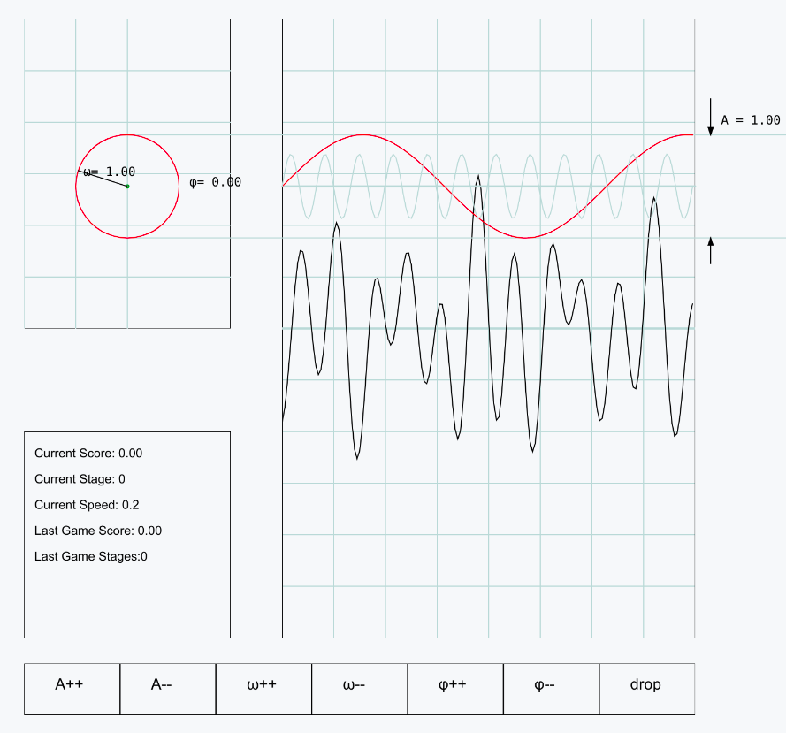
Sinusoids are flexible
The following animation is interactive. You can choose the values of \(A=\) , \(\omega=\) and \(\varphi=\) to plot the sinusoid (if you pick \(\varphi=\frac{\pi}{2}\) a cosine is plotted):
Sinusoids can be complex
Starting with the definition of a sinusoid:
\[y(t) = A * sin(2\pi ft + \varphi) = A * sin(\omega t + \varphi)\]If we multiply each side with \(A\):
\[A*e^{i\theta}=A*(\cos(\theta)+i*\sin(\theta))\]If we substitute \(\theta\) with \(\theta=\omega t + \varphi\) we obtain the complex sinusoid:
\[s(t)=A*e^{i(\omega t + \varphi)} = A * \cos(\underbrace{\omega t + \varphi}_{\theta}) + i * A * \sin(\underbrace{\omega t + \varphi}_{\theta})\]A complex sinusoid captures the behavior of two sinusoids (one cosine and one sine) on both its axes; on the real part, it behaves like a cosine, while on its imaginary part, it behaves like a sine.
The two are in sync as they both depend on the free variable \(\theta\), expressed as \(\theta=\omega t + \varphi\).
Two interesting observations:
- If we project the complex sinusoid on the plane determined by the Y-axis and Z-axis, we will plot a sine (the Imaginary part);
- If we project the complex sinusoid on the plane determined by the X-axis and Z-axis, we will plot a cosine (the Real part);
Sinusoids can nullify themselves
Two sinusoids in phase and sharing the same amplitude but with opposite frequencies nullify themselves.
Adding sinusoids leads to complexity
Let’s plot two arbitrary selected sinusoids \(y_{1}(x)\) and \(y_{2}(x)\), where:
- \(y_{1}(x) = \frac{9}{10} * sin(7x + \frac{\pi}{2})\), and
- \(y_{2}(x) = \frac{12}{10} * sin(3x - 2)\) .
The sum \(y(x)=y_{1}(x) + y_{2}(x)\) shows an interesting pattern
Adding random sinusoids for fun
Adding more sinusoids to an existing one (\(A=1\), \(\omega=1\), \(\varphi=1\)) generate more complex patterns:
Playing Sinusoidal tetris for fun
Not so long ago, I’ve re-imagined the game of Tetris.
It’s now possible to play Tetris with Sinusoids:
A square wave and sinusoids
If we carefully choose the sinusoids, we can create predictable patterns:
Let’s take, for example, use the following formula:
\[y(x) = \frac{4}{\pi}\sum_{k=1}^{\infty}\frac{\sin(2\pi(2k-1)fx)}{2k-1}\]Through expansion, the formula becomes:
\[y(x) = \underbrace{\frac{4}{\pi}\sin(\omega x)}_{y_{1}(x)} + \underbrace{\frac{4}{3\pi}\sin(3\omega x)}_{y_{2}(x)} + ... + \underbrace{\frac{4}{(2k-1)\pi}{\sin((2k-1)\omega x)}}_{y_k(x)} + ...\]\(y_1(x), y_2(x), y_3(x), ..., y_k(x), ...\) are all the individual sinusoids.
If we perform the sum, we will create a square wave. The more sinusoids we pick, the better the approximation.
Please choose how many sinusoids you want to use, and let’s see how the functions look like for (and \(\omega\)=):
Epicycles - First Encounter
One sinusoid has a corresponding circle that spins. So, the above animation can be re-imagined like this:
Pick and \(\omega\)= to plot the circles and the corresponding \(y_k(x)\) functions:
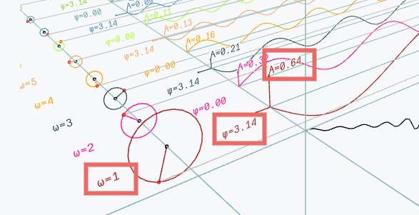
Epicycles - An intuitive understanding
There’s an intuitive proof to this: each epicycle corresponds to a specific sinusoid; when we talk about combining the sinusoids, we are talking about summing their positions at each point in time, and eventually, this operation reduces to subsequent vector additions.
Let’s take a simple example by introducing three arbitrarily picked sinusoids and their associated point vectors (or position vectors):
- \(y_{1}(x)=1.4sin(x + 1)\), with the associated position vector \(\vec{u_{1}}\);
- \(y_{2}(x)=0.8sin(2*x)\), with the associated position vector \(\vec{u_{2}}\);
- \(y_{3}(x)=0.5sin(3*x)\), with the associated position vector \(\vec{u_{3}}\).
Their sum is \(y(x) = y_{1}(x) + y_{2}(x) + y_{3}(x) = 1.4sin(x + 1) + =0.8sin(2*x) + 0.5sin(3*x)\).
A position vector represents the displacement from the origin \((0, 0)\) to a specific point in space. In our case, the vector \((x, y_{k}(x))\) represents the position or location of a point on the graph of the function(s) \(y_{k}(x)\) at a particular \(x\) value.
If we plot \(y(x)\) on the cartesian grid we obtain something like:
At each given point \(x\), we can say for certain that \(\vec{u} = \vec{u_{1}} + \vec{u_{2}} + \vec{u_{3}}\).
Epicycles - A flower
If we carefully pick the right sinusoids the moving circles can describe (approximate) any shape we want.
Here is a flower for example:
Can you guess the individual sinusoids working together to draw the flower?
You probably can’t unless you apply methods from a branch of mathematics called Fourier Analysis.
Fourier Series
Fourier Series is the mathematical process through which we expand a periodic function of period \(P\) as a sum of trigonometric functions.
Do you remember the Pink Floyd’s album cover for the Dark Side of The Moon:
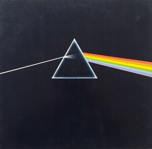
Imagine our function \(f(x)\) is the light itself, the prism is essentially Fourier Mathematics, and the spectral colors emanating from the prism are the sinusoids.
Following the analogy the formula looks like this:
\[\underbrace{f(x)}_{\text{ light itself}}=\underbrace{A_{0} + \sum_{n=1}^{\infty} [A_{n} cos(\frac{2\pi nx}{P}) + B_{n} sin(\frac{2\pi nx}{P})]}_{\text{the spectral components}}\]Where \(A_{n}\) and \(B_{n}\) are called Fourier Coefficients are defined by the following integrals:
\[A_{0} = \frac{1}{P} \int_{- \frac{P}{2}}^{+\frac{P}{2}} f(x) dx\] \[A_{n} = \frac{2}{P} \int_{- \frac{P}{2}}^{+ \frac{P}{2}} f(x) * \cos(\frac{2\pi nx}{P}) dx\] \[B_{n} = \frac{2}{P} \int_{- \frac{P}{2}}^{+ \frac{P}{2}} f(x) * \sin(\frac{2\pi nx}{P}) dx\]Fourier Series in Exponential Form
With the help of Euler’s Formula and by changing the sine and cosine functions in their exponential forms, we can also express the Fourier Series of a function as a sum of Complex Sinusoids:
\[f(x) = \sum_{n=-N}^{N} C_{n} e ^ {i2\pi \frac{n}{P}x}\]Where:
\[C_{n} = \begin{cases} A_{0} & \text{if } n = 0 \\ \frac{1}{2} (A_{n} - i * B_{n}) & \text{if } n > 0 \\ \frac{1}{2} (A_{n} + i * B_{n}) & \text{if } n < 0 \\ \end{cases}\]If we do additional substitutions, the final form of \(C_{n}\) is:
\[C_{n} = \frac{1}{P} \int_{-\frac{P}{2}}^{\frac{P}{2}} e^{-i2\pi\frac{n}{P}x} f(x) dx\]Example: The Fourier Series for the Box Function
Remember the Square Wave we’ve approximated with sinusoids in this section? At that point, we used the following formula to express the Square as a sum of sinusoidal components:
\[y(x) = \frac{4}{\pi}\sum_{k=1}^{\infty}\frac{\sin(2\pi(2k-1)fx)}{2k-1}\]Or, to keep things simpler, by substituting \(\omega=2\pi f\) (\(\omega\) is the angular frequency):
\[y(x) = \frac{4}{\pi}\sum_{k=1}^{\infty}\frac{\sin((2k-1)\omega x)}{2k-1}\]It’s time to understand how we’ve devised such an approximation.
In isolation, the Square Wave, \(f(x)\) looks like this:
Throughout the interval [0, 2L], \(f(x)\) can be written as:
Where \(H(x)\) is called the Heavisde Step Function and has the following definition:
\[H(x) = \begin{cases} 0 & \text{if } x \lt 0 \\ 1 & \text{if } x \ge 0 \\ \end{cases}\]First of all, let’s look at \(A_{0} = \frac{1}{2L} \int_{0}^{2L} f(x) dx\). Notice how we’ve changed the interval from \([-\frac{P}{2}, \frac{P}{2}]\) to \([0, 2L]\) to match our example. This will be reflected in the formulas.
Well, this coefficient (\(A_{0}\)) is a fancy way to express the average of \(f(x)\) over the interval (in our case [0, 2L]). In the same time \(A_{0}\) is the area determined by \(f(x)\) over [0, 2L] then divided by \(2L\). But if you look at the plot again, you will see that the net area is \(0\), because the green area (S1) nullifies the red area (S2), regardless of \(L\).
Secondly, let’s compute the \(A_{n} = \frac{1}{L} \int_{0}^{2L} f(x) * \cos(\frac{\pi nx}{L}) dx\) coefficients. An important observation is that \(f(n)\) is odd, and its average value on the interval is \(0\); we can safely say all the coefficients \(A_{n}\) also vanish.
Visually speaking, regardless of how you pick \(n\) or \(L\), the net area determined by the \(A_{n}\) integral will always be zero. It’s visually obvious if we plot \(A_n\). For example plotting \(A_{1}\), \(A_{2}\), \(A_{3}\), \(A_{4}\) looks like this:
Similar symmetrical patterns will emerge if you increase the \(n\) in \(A_{n}\) and plot them.
Thirdly, we need to compute:
\[B_{n} = \frac{1}{L} \int_{0}^{2L} f(x) * \sin(\frac{\pi nx}{L}) dx\]If we plot a \(B_{1}\), \(B_{2}\), \(B_{3}\) and, let’s say, \(B_{4}\) we can intuitively feel what’s happening with \(B_{n}\):
If you have a keen eye for geometrical representations, you will notice that every even \(B_{n}\) is also 0. The red and green areas nullify, so the net area described by the integral is \(0\). The odd terms will be \(2 * \text{something}\), so let’s calculate that \(\text{something}\).
We will need to split the integral on two sub-intervals \([0, L]\) and \([L, 2L]\) (there’s a chasm at \(L\)), but given the fact \(f(x)\) and \(sin(x)\) are odd, \(B_{n}\) can we written as:
\[B_{n} = 2 * [\frac{1}{L} \int_{0}^{L} f(x) * \sin(\frac{\pi nx}{L}) dx]\]We can now perform u-substition, so we can write:
\[B_{n} = \frac{2}{L} \int_{0}^{nL\pi} \frac{\sin(\frac{u}{L})}{n\pi}du\]After we take the constant out, we compute the integral, use the intervals, and take into consideration the periodicity of cosine:
\[B_{n} = \frac{2}{n\pi}(1-(-1)^n)\]And now we see it, \(B_{n}\) is exactly \(0\) if \(n\) is even, and \(B_{n}=2 * \frac{2}{n\pi}\) is \(n\) is odd.
Putting all back into the master formula of the Fourier Series:
\[f(x)=\underbrace{A_{0}}_{0} + \sum_{n=1}^{\infty} [\underbrace{A_{n} \cos(\frac{\pi nx}{L})}_{0} + B_{n} \sin(\frac{\pi nx}{L})]\]Things become:
\[f(x)=\frac{4}{\pi} \sum_{n=1,3,5...}^{+\infty} (\frac{1}{n} * \sin(\frac{\pi nx}{L}))\]If we substitute \(n \rightarrow 2k-1\) and consider, we obtain the initial formula:
\[f(x)=\frac{4}{\pi} \sum_{k=1}^{+\infty} (\frac{\sin(\frac{\pi (2k-1)x}{L})}{(2k-1)})\]To obtain the initial formula, we substitute \(L \rightarrow \frac{1}{2f}\), and \(2\pi f \rightarrow \omega\), basically we create an interdependence between \(L\) (half of the interval) and \(\omega\), \(L=\frac{\pi}{\omega}\):
\[f(x) = \frac{4}{\pi}\sum_{k=1}^{\infty}\frac{\sin((2k-1)\omega x)}{2k-1}\]Unfortunately, there’s no way we can go to \(+\infty\), so let’s consider \(s(x)\) as an approximation of \(f(x)\) that depends on \(n\).
\[s(x) = \frac{4}{\pi}\sum_{k=1}^{n}\frac{\sin((2k-1)\omega x)}{2k-1} \approx f(x)\]In the next animation, you will see that by increasing \(n\), the accuracy of our approximation gets better and better, and the gaps are slowly closed:
To understand how adding more coefficients improves the approximation, let’s look back again at a few of our coefficients \(s_{1}(x)\), \(s_{2}(x)\), \(s_{3}(x)\), \(s_{4}(x)\) and \(s_{5}(x)\) (we will pick \(\omega=\frac{\pi}{2}\), so that \(2L=1\)):
\[s_{1}(x) = \frac{4}{\pi} \sin(\frac{\pi x}{2})\] \[s_{2}(x) = \frac{4}{3\pi} \sin(\frac{3\pi x}{2})\] \[s_{3}(x) = \frac{4}{5\pi} \sin(\frac{5\pi x}{2})\] \[s_{4}(x) = \frac{4}{7\pi} \sin(\frac{7\pi x}{2})\] \[s_{5}(x) = \frac{4}{9\pi} \sin(\frac{9\pi x}{2})\]Each of the 5 terms is a sinusoid, with \(\frac{4}{\pi}\), \(\frac{4}{3\pi}\), etc. amplitudes, and \(\frac{\pi}{2}\), \(\frac{3\pi}{2}\), etc. frequencies.
So, if we were to approximate a Square Wave with its fifth partial sum (the red dot), we would obtain something like this:
Notice how obsessed the red dot is with the blue dot (the actual function) and how closely it follows it.
We can always add more terms to the partial sum to help the red dot in its holy mission, improving the approximation until nobody cares anymore.
Example - The Fourier Series of the Triangle wave
Without dealing with all the associated math, the Fourier Series decomposition for a triangle-wave is:
\[s(x)=\frac{8}{\pi^2}\sum_{k=1}^{N}\frac{(-1)^{k-1}}{(2k-1)^2}*\sin((2k-1)x)\]Plotting the function \(s(x)\), we will see that things converge smoothly and fast. As soon as \(n\) approaches \(6\), we can already observe the triangle:
Let’s compute the first terms six terms of the \(\sum\), so that:
\[s(x) \approx s_1(x) + s_2(x) + s_3(x) + s_4(x) + s_5(x) + s_6(x)\]Where:
- The first term is \(s_1(x)=\frac{8}{\pi^2}*\sin(x)\), where \(A=\frac{8}{\pi^2}\), \(\omega=1\), \(\varphi=0\);
- The second term is \(s_2(x)=-\frac{8}{3^2\pi^2}*\sin(3x)\), where \(A=-\frac{8}{3^2\pi^2}\), \(\omega=3\), \(\varphi=0\);
- The third term is \(s_3(x)=\frac{8}{5^2\pi^2}*\sin(5x)\), where \(A=\frac{8}{5^2\pi^2}\), \(\omega=5\), \(\varphi=0\);
- The fourth term is \(s_4(x)=-\frac{8}{7^2\pi^2}*\sin(7x)\), where \(A=-\frac{8}{7^2\pi^2}\), \(\omega=7\), \(\varphi=0\);
- The fifth term is \(s_5(x)=\frac{8}{9^2\pi^2}*\sin(9x)\), where \(A=\frac{8}{9^2\pi^2}\), \(\omega=9\), \(\varphi=0\);
- The sixth term is \(s_6(x)=-\frac{8}{11^2\pi^2}*\sin(11x)\), where \(A=-\frac{8}{11^2\pi^2}\), \(\omega=11\), \(\varphi=0\);
A keen eye will see will observe the that \(s_2(x)\), \(s_4(x)\), \(s_6(x)\) and all the even terms are negative.
A negative amplitude doesn’t make too much sense, at least not in a physical sense. What are we going to do with the minus sign?
We have two options:
- Because \(\sin(-x)=-\sin(x)\), nobody stops us to make the frequency negative. For example, \(s_2(x)=\frac{8}{3^2\pi^2}*\sin(-3x)\), so that the \(\omega=-3\). But again, why would we want a negative frequency? This also doesn’t make sense in a physical sense.
- We can use \(\vert A \vert\) and shift the signal with \(\pi\), so that \(\varphi=\pi\).
In practice, we will go with 2. as it’s more practical and gives us more control, but the two options are equivalent so that we can write \(s_2(x)\) in both ways:
\[s_2(x)=-\frac{8}{3^2\pi^2}*\sin(3x)\] \[s_2(x)=\frac{8}{3^2\pi^2}*\sin(3x + \pi)\]Visually speaking, the results will not be surprising if we plot \(sin(-x)\) and \(sin(x+\pi)\) side by side; the two are equivalent:
If we consider this, the even terms of \(s(x)\) will become:
- \(s_2(x)=\frac{8}{3^2\pi^2}*sin(3x+\pi)\) ;
- \(s_4(x)=\frac{8}{7^2\pi^2}*sin(7x+\pi)\) ;
- \(s_6(x)=\frac{8}{11^2\pi^2}*sin(11x+\pi)\) ;
- …and so on
Example - The Fourier Series of a Sawtooth Function
Shamelessly skipping the math demonstration, a reverse-sawtooth function has the following form:
\[s(x)=\frac{2}{\pi}\sum_{k=1}^{N}(-1)^k*\frac{\sin(kx)}{k}\]Plotting \(s(x)\), while increasing \(n\), things look like this:
The Fourier Series Machinery
To better visualize what’s happening, let’s look at a Fourier Series Machinery and how the circles move to create beautiful practical patterns.
You can pick the shape of the desired signal from here: and the sketch will change accordingly.
…A bunch of spinning circles on a stick, where each circle corresponds to exactly one term of the series - this is the marvelous Fourier Series Machinery.
If we run our signal through the Fourier Series Machinery, we will obtain The Amplitude (\(A\)) and The Phase (\(\varphi\)) for each Frequency (\(\omega\)) from \(1\) to \(N\). Isn’t it amazing? And it all comes down to a bunch of spinning circles… on a stick.
to be continued
Comments