A tale of Java Hash Tables
The intended audience for this article is undergrad students who already have a good grasp of Java, or seasoned Java developers who would like to explore an in-depth analysis of various hash table implementations that use Open Addressing.
The reader should be familiar with Java generics, collections, basic data structures, hash functions, and bitwise operations.
Introduction
In Java, the primary hash table implementation, HashMap<K,V>, employs the classical Separate Chaining technique with its critical optimizations (such as treeifying bins) to reduce read times during high-collision scenarios.
However, the choice between Separate Chaining and Open Addressing is a point of divergence among programming language designers.
As analyzed in this deep dive, languages like Python, Ruby, and Rust favor Open Addressing for their standard dictionaries, while Java, Go, C#, and C++ remain more conservative, sticking to Separate Chaining.
Standard Implementations by Language
| Programming Language | Hash Table Algorithm | Source(s) |
|---|---|---|
| Python | Open Addressing | dictobject.c |
| Ruby | Open Addressing | st.c |
| Rust | Open Addressing | map.rs |
| Java | Separate Chaining | HashMap.java |
| Go | Separate Chaining | maphash.go |
| C# | Separate Chaining | Dictionary.cs |
| C++ | Separate Chaining | hashtable.h |
Objectives and Scope
In this article, we will explore how to implement hash tables in Java using various Open Addressing strategies. We will then benchmark these custom implementations against the reference HashMap<K,V>.
- Design Choices: I have intentionally skipped Quadratic Probing, as I find Python’s “perturbation” approach more sophisticated. While I drew inspiration from Hopscotch Hashing, I’ve implemented a variation rather than the pure algorithm. A draft of Cuckoo Hashing is also available in the repository for the curious.
- Academic Context: These implementations are academic in nature. While a developer specialized in low-level Java optimization could likely push these further, these serve as a clear baseline for structural comparison.
- Benchmarking: Measuring performance in the JVM is notoriously tricky. I have used JMH (Java Microbenchmark Harness) to ensure results are as accurate as possible, but I welcome feedback on the methodology.
The Contenders
We will implement and benchmark six Map<K,V> variations against HashMap<K,V>:
| Java Class | Source | Description |
|---|---|---|
LProbMap<K, V> | src | A classic Open Addressing implementation using Linear Probing. |
LProbSOAMap<K,V> | src | A “Structure of Arrays” (SOA) approach to linear probing, optimizing memory layout for cache locality. |
LProbBinsMap<K,V> | src | An implementation inspired by Ruby’s hash table design. |
LProbRadarMap<K, V> | src | Uses a separate bit-vector (“radar”) to track item locations, similar to Hopscotch Hashing. |
PerturbMap<K, V> | src | Implements Python’s perturbation algorithm to resolve collisions more effectively than simple linear steps. |
RobinHoodMap<K, V> | src | Robin Hood Hashing: a linear probing variant that minimizes variance in probe lengths. |
Getting Started
The full source code is available on GitHub:
git clone git@github.com:nomemory/open-addressing-java-maps.git
Before we dive into the Java code, I highly recommend reviewing my previous article on C-based hash tables. It provides a necessary refresh on theoretical fundamentals, such as hash functions and load factors, which remain constant regardless of the language.
Separate Chaining, or how HashMap<K,V> works internally
As I’ve previously stated, HashMap<K,V> is implemented using a typical Separate Chaining technique. If you jump straight into reading the source code, things can be a little confusing, especially if you don’t know what you are looking for. But once you understand the main concepts, everything becomes much clearer.
Even if this is not the primary purpose of this article, I believe it’s always a good idea to understand how
HashMap<K,V>works. Many Java interviewers love to ask this question!
If you already understand how HashMap<K,V> works, you can skip directly to the next section. If you don’t, and you are curious about it, please read on.
The Table and the Nodes
The HashMap<K,V> class contains an array of Node<K,V>. For simplicity, we are going to call this array table:
// The table, initialized on first use, and resized as necessary.
// When allocated, length is always a power of two.
transient Node<K,V>[] table;
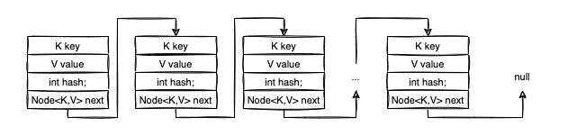
The table is the most important structure in the class; it’s the actual space where we store our data. Each entry in this array is a Node<K,V>, which has the following composition:
static class Node<K,V> implements Map.Entry<K,V> {
        final int hash;
        final K key;
        V value;
        Node<K,V> next;

        // getters and setters + other goodies
}
As you likely noticed, Node<K,V> is used to implement a linked data structure. The next attribute references the next Node in the chain. Think of the Node<K,V>[] table as an array of linked structures, for simplicity, let’s assume those chained structures are linked lists.
Mapping Cities: An Example
To make things transparent, let’s define a HashMap<String, String>, where keys K are European capital cities and values V are the corresponding countries.
Initially, the table is empty with a default capacity of 1 << 4 (which equals 16). The choice of using a power of two is not accidental, as we will see shortly.
Now, let’s insert our first entries: <"Paris", "France">, <"Sofia", "Bulgaria">, <"Madrid", "Spain">, and <"Bucharest", "Romania">.
When you call put(K key, V value), the call is dispatched to putVal(...):
public V put(K key, V value) {
    return putVal(hash(key), key, value, false, true);
}
Before putVal runs, the VM must compute hash(key). HashMap accepts null keys, which by convention always hash to 0. For everything else, it uses this bit-shifting logic:
static final int hash(Object key) {
    int h;
    return (key == null) ? 0 : (h = key.hashCode()) ^ (h >>> 16);
}
The extra bitwise operation improves the diffusion of the hashCode() by mixing higher-order bits into the lower ones. This reduces collisions. Applying this to our cities, we get:
- Paris: 76885502
- Sofia: 80061639
- Madrid: -1997818570
- Bucharest: -543452922
The “Magic” of Bucket Indexing
In putVal, the map identifies the correct bucket using: tab[i = (n - 1) & hash].
Because n (table length) is always a power of two, (n - 1) & hash is a mathematical shortcut for hash % n. It “projects” the massive range of integer values into our specific array indices {0, 1, ..., n-1} while avoiding the slow modulo operator.
Calculating our indices:
- Paris: (16-1) & 76885502 = 14
- Sofia: (16-1) & 80061639 = 7
- Madrid: (16-1) & -1997818570 = 6
- Bucharest: (16-1) & -543452922 = 6
Notice that Madrid and Bucharest both want to go to index 6. This is a hash collision.

- Paris is stored at
table[14]. - Sofia is stored at
table[7]. - Madrid is stored at
table[6]. - Bucharest also maps to
table[6]. Since the slot is occupied, the new node is appended to the chain (Madrid’snextnow points to Bucharest).
Retrieval: Following the Trail
Retrieving an element with get("Bucharest") follows the same path:
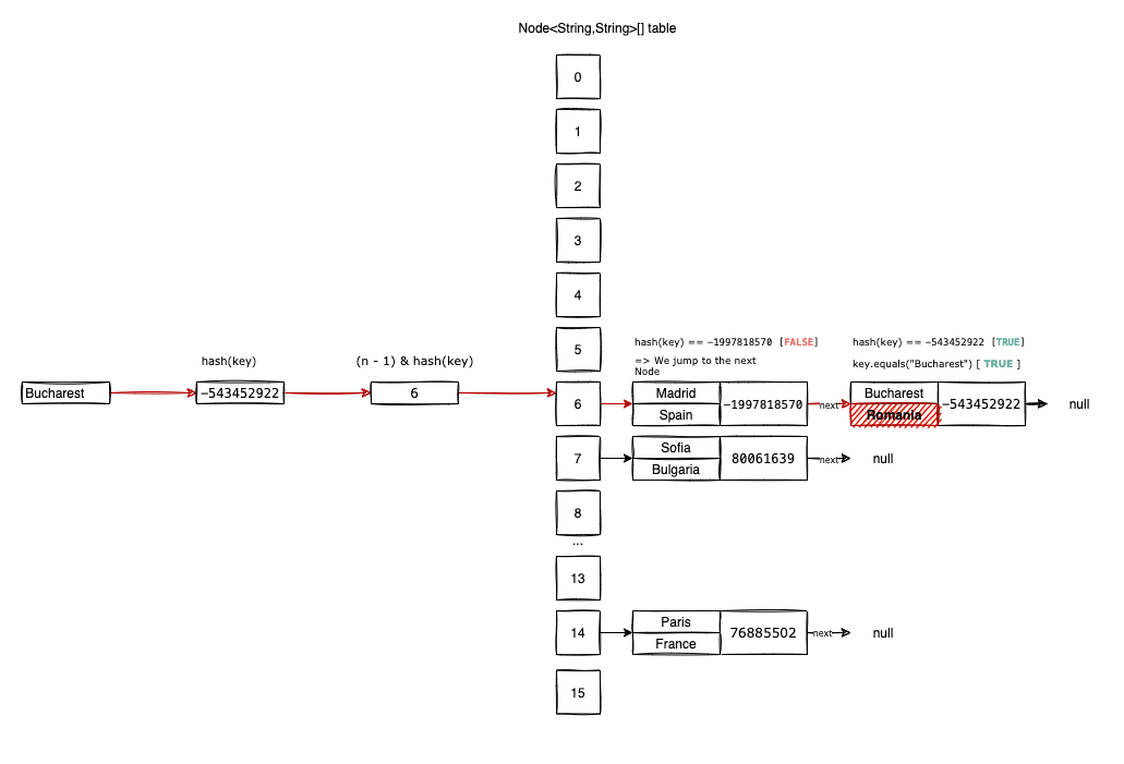
- Compute
hash("Bucharest"). - Find index 6.
- Compare the hash and key of the first node at
table[6](Madrid). - Since they don’t match, follow
nextto the next node. - Check if
"Bucharest".equals(currentNode.key). If true, return the value.
Performance Optimizations
HashMap isn’t just a simple array of lists; it performs two vital optimizations:
1. Capacity Adjustment (Resizing)
The loadFactor (default 0.75) defines when to resize. If you have 16 slots and insert 13 items, $13/16 > 0.75$. The map will double its capacity to 32 and rehash every existing element. This keeps the chains short and the lookup time close to $O(1)$.

2. Bucket Adjustment (Treeification)
If a single bucket’s chain becomes too long (reaching TREEIFY_THRESHOLD = 8), HashMap converts that linked list into a Red-Black Tree. This changes the worst-case search time from $O(n)$ to $O(\log n)$, preventing performance degradation even during heavy collisions.

Open Addressing
Compared to Separate Chaining, Open Addressing hash tables store only one entry per slot. There are no real buckets, no linked lists, and no red-black trees. Instead, the implementation relies on a single, extensive array that contains everything the map needs to operate.
If the array of pairs is sparse enough (typically operating at a load factor $< 0.77$) and the hashing function provides decent diffusion, hash collisions should be rare. However, they are still inevitable. When a collision occurs, we “probe” the array to find another available slot for the entry.
The most straightforward probing algorithm is linear probing. In the event of a collision, we iterate through each subsequent slot (starting from the initially computed index) until we find an empty spot for insertion. If we reach the end of the array, we simply wrap around to index 0.
The primary advantage of Open Addressing over Separate Chaining is the reduction of cache misses. Because the data resides in a single contiguous block of memory, the CPU can leverage spatial locality much more effectively.

The biggest shortcoming of Open Addressing is its sensitivity to sub-optimal hash functions. Consider an extreme case: a hash function that returns a constant value. In this scenario, every element targets the same slot, leading to a collision for every insertion.
While HashMap<K,V> would gracefully degrade to $O(\log n)$ performance (thanks to its treeified buckets), a Linear Probing implementation would degrade to $O(n)$, effectively becoming a very slow linked list.

In practice, few developers use a constant-returning hash function, but even mildly sub-optimal functions lead to clustering. This is a phenomenon where occupied slots form dense groups, forcing the VM to traverse long sequences during every insert, read, or delete operation.
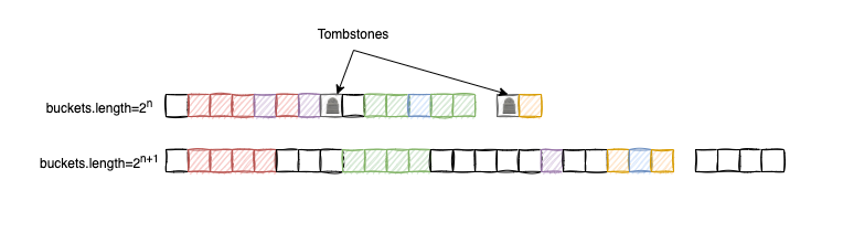
Tombstones
Deleting an element from an Open Addressing table is a subtle task. We cannot simply set a slot to null because doing so might break a probing sequence, making subsequent elements “unreachable” during a search. To solve this, we use tombstones.
Whenever an entry is deleted, we mark the slot with a special “tombstone” flag:
- Inserts: A tombstone is treated as an empty slot and is a candidate for a new entry.
- Reads/Deletes: We skip the tombstone and continue the traversal to ensure we don’t miss elements further down the probe sequence.
When resizing the array, we filter out these tombstones to clean up the “junk” left behind by deletions. While algorithms that avoid tombstones exist (involving complex element shifts), I’ve opted for the tombstone approach because deletions are typically rare in most Map use cases, and their impact on performance is generally negligible.
LProbMap<K, V>
LProbMap<K,V> is my initial “academic” attempt at implementing an Open Addressing map in Java. This implementation follows the standard algorithms “by the book” without excessive micro-optimizations.
You can find the full source code for this implementation here.
The class extends Map<K,V>, requiring an implementation for all standard interface methods. Let’s look at the core structure and the primary put method:
public class LProbMap<K, V> implements Map<K,V> {

    private static final double DEFAULT_MAX_LOAD_FACTOR = 0.6;
    private static final double DEFAULT_MIN_LOAD_FACTOR = DEFAULT_MAX_LOAD_FACTOR / 4;
    private static final int DEFAULT_MAP_CAPACITY_POW_2 = 6;

    private int size = 0;
    private int tombstones = 0;
    private int capPow2 = DEFAULT_MAP_CAPACITY_POW_2;

    public LProbMapEntry<K, V>[] buckets =
                        new LProbMapEntry[1 << DEFAULT_MAP_CAPACITY_POW_2];

    // ... additional logic ...
}
The DEFAULT_MAX_LOAD_FACTOR is set to 0.6. Once the map reaches this threshold, it triggers a resize. While this leaves 40% of the array empty, it significantly improves read performance by keeping probe sequences short. The load factor is calculated as: (size + tombstones) / buckets.length.
The Hash Function
We use a “finalizer” inspired by Murmur Hash to improve the diffusion of Java’s native hashCode():
public static int hash(final Object obj) {
    int h = obj.hashCode();
    h ^= h >> 16;
    h *= 0x3243f6a9;
    h ^= h >> 16;
    return h & 0xfffffff; // Ensure the result is non-negative
}
The bitwise & 0xfffffff ensures we don’t deal with negative indices, as Java lacks an unsigned 32-bit integer type.
Inserting an Entry
The insertion logic for LProbMap follows these steps:
- Increase capacity if the load factor threshold is exceeded.
- Calculate the base slot using the hash.
- If the slot is
null, insert the entry. - If the slot is occupied, use linear probing (step through the array) until we find a tombstone, an empty slot, or the existing key.
Note: Our convention uses entries with null keys to represent tombstones, so this map does not support null keys.
protected V put(K key, V value, int hash) {
    increaseCapacity();
    int idx = hash & (buckets.length - 1); // The "Base Slot" calculation

    while(true) {
        if (buckets[idx] == null) {
            buckets[idx] = new LProbMapEntry<>(key, value, hash);
            size++;
            return null;
        }
        else if (buckets[idx].key == null) { // Found a tombstone
            buckets[idx].key = key;
            buckets[idx].value = value;
            buckets[idx].hash = hash;
            size++;
            tombstones--;
            return null;
        }
        else if (buckets[idx].hash == hash && key.equals(buckets[idx].key)) {
            V ret = buckets[idx].value;
            buckets[idx].value = value;
            return ret;
        }

        // Linear probing: jump to the next index or wrap around
        idx++;
        if (buckets.length == idx) idx = 0;
    }
}
The Bitwise Modulo Trick
The line int idx = hash & (buckets.length - 1) is a common optimization. In computer architecture, the modulo operator (%) is relatively expensive compared to bitwise operations.
Since our table size is always a power of two ($2^n$), we can use a bitwise AND with a mask of all ones ($2^n - 1$) to calculate the remainder. This is effectively “cutting” the number to fit the array size.
[Image explaining the bitwise AND mask as a modulo shortcut]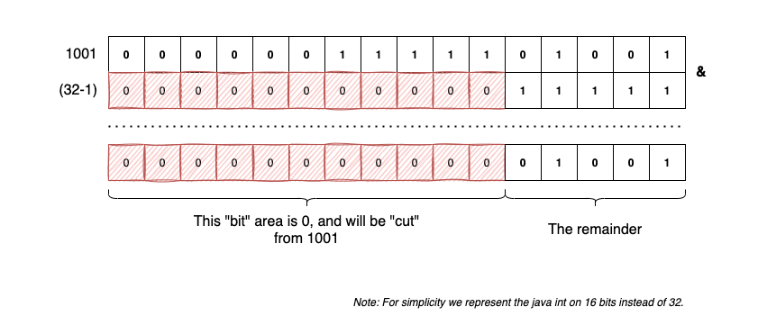
Retrieving an Entry
The algorithm for retrieving a value by its key follows the same probing logic used during insertion. The process is as follows:
- Compute the
hash(key). - Calculate the base slot:
idx = hash & (buckets.length - 1). - If the base slot is
null, we are 100% certain the key does not exist in the map, and we returnnull. - If the slot is occupied, we check if the stored
hashmatches our key’shash.- If hashes match, we perform a final
equals()check to account for potential hash collisions. - If they match, we return the value.
- If they don’t match (or if we encounter a tombstone), we probe further using linear probing.
- If hashes match, we perform a final
- We repeat this until we either find the key or encounter a
nullslot, which signifies the end of the cluster.
public V get(Object key) {
    int hash = hash(key);
    int idx = hash & (buckets.length - 1);
    LProbMapEntry<K,V> bucket = buckets[idx];

    if (bucket == null) {
        return null;
    }

    do {
        // Match found: check hash first (fast), then equals()
        if (bucket.hash == hash && key.equals(bucket.key)) {
            return bucket.value;
        }
        // Linear probing: wrap around if at the end of the array
        idx++;
        if (idx == buckets.length) idx = 0;
        bucket = buckets[idx];
    } while(bucket != null);

    return null;
}
Deleting an Entry
Deletion in an Open Addressing table requires care to avoid breaking the “chain” of a cluster. Instead of nullifying a slot, we replace the entry with a tombstone (represented here by setting the key to null within an existing entry).
- Identify the base slot for the key.
- If the base slot is
null, the key isn’t here; returnnull. - Otherwise, probe through the cluster comparing hashes and keys.
- When the element is found:
- Remove it by marking the slot as a tombstone.
- Increment the
tombstonescounter and decrement thesize. - Return the old value.
- After the operation, check if the load factor has dropped enough to justify decreasing the table capacity.
public V remove(Object key) {
    int hash = hash(key);
    int idx = hash & (buckets.length - 1);

    if (buckets[idx] == null) {
        return null;
    }

    do {
        if (buckets[idx].hash == hash && key.equals(buckets[idx].key)) {
            V oldVal = buckets[idx].value;
            // Mark as tombstone: clear key/value but keep the slot non-null
            buckets[idx].key = null;
            buckets[idx].value = null;
            buckets[idx].hash = 0;
            tombstones++;
            size--;

            decreaseCapacity();
            return oldVal;
        }
        idx++;
        if (idx == buckets.length) idx = 0;
    } while (buckets[idx] != null);

    return null;
}
Resizing and Rehashing
We follow a similar strategy to HashMap<K,V> for capacity management. If the load factor (including tombstones) exceeds our maximum threshold, we double the capacity. Conversely, if the load factor falls below a minimum threshold, we halve it.
Capacity adjustment is crucial for two reasons:
- Clustering Control: It breaks up dense clusters that degrade performance.
- Tombstone Cleanup: Since we don’t rehash tombstones, resizing effectively purges the “junk” elements from our memory, making the array sparse again.
protected final void reHashElements(int capModifier) {
    this.capPow2 += capModifier;
    LProbMapEntry<K, V>[] oldBuckets = this.buckets;

    // Allocate new array with updated power-of-two capacity
    this.buckets = new LProbMapEntry[1 << capPow2];
    this.size = 0;
    this.tombstones = 0;

    // Full rehash: re-insert all non-deleted elements
    for (int i = 0; i < oldBuckets.length; ++i) {
        if (oldBuckets[i] != null && oldBuckets[i].key != null) {
            // Re-insert using the new capacity
            this.put(oldBuckets[i].key, oldBuckets[i].value, oldBuckets[i].hash);
        }
    }
}

protected final void increaseCapacity() {
    final double lf = (double)(size + tombstones) / buckets.length;
    if (lf > DEFAULT_MAX_LOAD_FACTOR) {
        reHashElements(1);
    }
}

protected final void decreaseCapacity() {
    final double lf = (double)size / buckets.length;
    if (lf < DEFAULT_MIN_LOAD_FACTOR && this.capPow2 > DEFAULT_MAP_CAPACITY_POW_2) {
        reHashElements(-1);
    }
}
While this implementation is functional, it could be further optimized by pre-calculating the threshold values (e.g., maxSize = capacity * loadFactor) to avoid floating-point division during every put or remove call.
LProbSOAMap<K,V>
This implementation follows a nice optimization proposed by dzaima on GitHub, focusing on memory layout and allocation overhead.
For the full source code, please check the repository link.
The core argument for this approach centers on how Java handles object allocation and cache locality:
“A very important property of open addressing is the ability to avoid an allocation per inserted item. Without that,
LProbMapand Java’sHashMapdiffer only by where the next object pointer is read a list inLProbMapor the entry object inHashMap. Since both are likely already in cache, performance remains similar. To truly leverage Open Addressing in Java, we should utilize a Struct-of-Arrays approach.”
By moving away from an array of entry objects (Array of Structures), we can eliminate the overhead of creating a new Map.Entry object for every single insertion. While Java doesn’t yet have native “value types” (like C# structs), we can simulate a flatter memory layout by splitting the entry components into primitive and object arrays.
In LProbSOAMap, we discard the LProbMapEntry<K, V>[] buckets array. Instead, we distribute the keys, values, and hashes across three distinct, parallel arrays:
public K[] bucketsK = (K[]) new Object[1 << DEFAULT_MAP_CAPACITY_POW_2];
public V[] bucketsV = (V[]) new Object[1 << DEFAULT_MAP_CAPACITY_POW_2];
// hash=0 indicates empty; hash=1 indicates a tombstone
public int[] bucketsH = new int[1 << DEFAULT_MAP_CAPACITY_POW_2];
In the standard LProbMap, every time you add an element, you perform a new LProbMapEntry<>(...). This places pressure on the Garbage Collector and adds a layer of indirection (a pointer to an object).
By using the SoA approach:
- Zero Allocation on Put: We simply write the key and value references into existing array slots.
- Primitive Efficiency: The
int[] bucketsHstores hashes as raw primitives, which is much more cache-friendly than wrapping them in an object. - Sequential Access: During linear probing, the CPU can pre-fetch the next elements in these arrays more efficiently than it can traverse a chain of separate entry objects.
While this means the VM has to manage three separate memory locations, it remains one of the best ways to minimize the “object tax” in modern Java performance tuning.
PerturbMap<K, V>
The PerturbMap<K, V> is nearly identical to LProbMap<K, V>, but it introduces one significant change in how it handles collisions. Instead of relying on sequential steps, it uses a pseudo-random probing sequence.
While studying the CPython source code for the dict implementation, I came across a fascinating logic for resolving collisions:
“This is done by initializing an (unsigned) variable ‘perturb’ to the full hash code, and changing the recurrence to:
perturb >>= PERTURB_SHIFT;
j = (5 * j) + 1 + perturb;
use j % 2**i as the next table index;”
Scrambling the Search Path
To combat clustering, which happens when a mediocre hash function causes entries to “clump” together, Python proposes a strategy that doesn’t use linear probing. Instead, it “scrambles” the probing sequence to find the next index.
Instead of the simple cycle used in linear probing:
idx++;
if (idx == buckets.length) idx = 0;
We implement the Python-inspired recurrence:
idx = (5 * idx) + 1 + perturb;
perturb >>= SHIFTER;
idx = idx & (buckets.length - 1);
Here, SHIFTER is a constant (typically 5) and perturb is initialized to the original hash. As the loop progresses, perturb eventually reaches zero, and the algorithm settles into a deterministic sequence that still guarantees every slot will be visited.
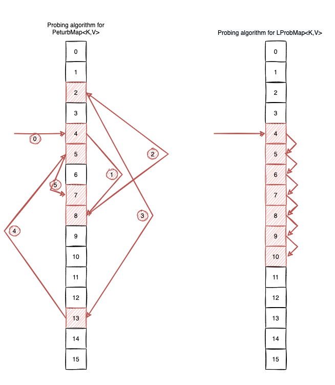
A Practical Example
Let’s assume an initial hash = 32132932, SHIFTER = 5, and a buckets.length = 16. If we encounter collisions, the probing sequence would jump like this:
final int hash = 32132932;
final int shifter = 5;
final int bucketsLength = 1 << 4;

int idx = hash & (bucketsLength - 1); // Initial: 4
int perturb = hash;
for(int j = 0; j < 5; j++) {
    idx = (5 * idx) + 1 + perturb;
    perturb >>= shifter;
    idx = idx & (bucketsLength - 1);
    System.out.print(idx + " ");
}
// Output: 8 2 13 5 7
Visually, this prevents a “clump” of data from forcing the CPU to read ten items in a row. Instead, the VM “jumps” across the array to find space.
Implementation of get(Object key)
The retrieval logic remains familiar, but with the updated indexing recurrence:
public V get(Object key) {
    if (null == key) throw new IllegalArgumentException("Null keys not supported");

    int hash = hash32(key);
    int idx = hash & (buckets.length - 1);

    if (buckets[idx] == null) return null;

    int perturb = hash;
    do {
        if (buckets[idx].hash == hash && key.equals(buckets[idx].key)) {
            return buckets[idx].value;
        }

        // The Scrambling Logic
        idx = (5 * idx) + 1 + perturb;
        perturb >>= SHIFTER;
        idx = idx & (buckets.length - 1);

    } while (buckets[idx] != null);

    return null;
}
Performance Trade-offs
- Clustering Defense: We effectively eliminate primary clustering by augmenting the hash function’s diffusion through the probing logic itself.
- Cache Locality: The trade-off is a potential increase in cache misses. Linear probing is fast because it reads contiguous memory;
PerturbMapjumps around, which may force the CPU to fetch new cache lines more frequently.
LProbBinsMap<K,V>
This implementation is closely related to LProbMap<K,V>, but introduces a structural change inspired by Ruby’s hash table implementation. To keep the comparison fair, I have continued to use linear probing as the search algorithm.
For the full source code, please check this link.
Separating Metadata from Data
The core concept is to decouple the probing logic from the actual data storage. Instead of one large array of objects, we split the information between two specialized arrays:
int[] bins: A sparse array of integers. Instead of storing entries directly, this array stores the indices of where the entries can be found.Map.Entry<K,V>[] entries: A dense,ArrayList-like structure. This is where the actual keys, values, and hashes are stored.
Visually, LProbBinsMap<K,V> organizes its memory like this:
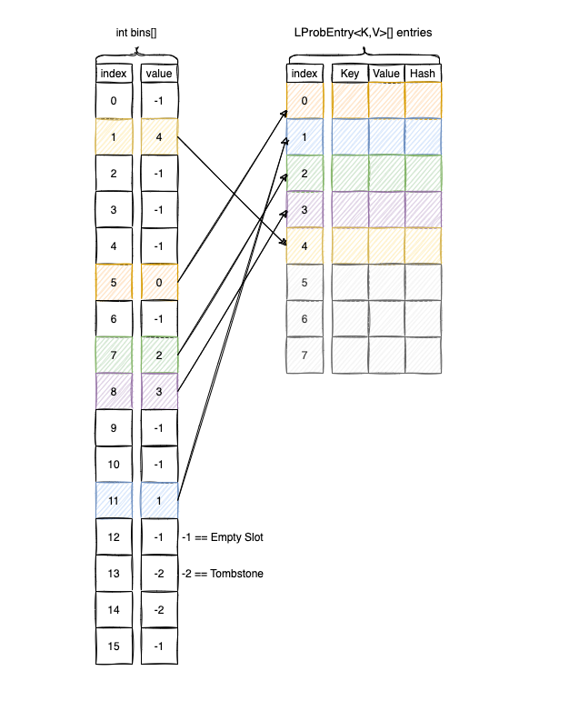
To find an element, we perform our hash-based lookup in the bins array first. The value found there serves as a pointer to the correct location in the entries array.
Implementation of get(Object key)
Coded as a re-interpretation of the standard linear probing logic, the get method looks like this:
public V get(Object key) {
    if (null == key) throw new IllegalArgumentException("Null keys not supported");

    int hash = hash(key);
    int idx = hash & (bins.length - 1);

    // If the bin is empty, we know the key doesn't exist
    if (bins[idx] == EMPTY_SLOT) {
        return null;
    }

    do {
        int entryIdx = bins[idx];
        // Skip tombstones and check the entry at the indexed position
        if (entryIdx != TOMBSTONE) {
            LProbMapEntry<K, V> entry = entries[entryIdx];
            if (entry.hash == hash && key.equals(entry.key)) {
                return entry.value;
            }
        }

        // Linear probing through the bins array
        idx++;
        if (idx == bins.length) idx = 0;

    } while (bins[idx] != EMPTY_SLOT);

    return null;
}
Advantages of the “Bins” Approach
- Reduced Memory Footprint: In a standard Open Addressing map, a sparse array of object references (
Entry[]) can be memory-intensive. In this model, the sparse array is just primitives (int[]), which is much smaller. - Dense Data Storage: The
entriesarray is packed densely. This improves cache locality when the VM needs to iterate over all elements (like during resizing or entry sets), as it doesn’t have to skip over large gaps ofnullslots. - Cache-Friendly Probing: Probing through an
int[]is incredibly fast. The CPU can fit many more “bins” into a single cache line than it can with “entry” objects, making the search for the correct index highly efficient.
LProbRadarMap<K, V>
LProbRadarMap<K, V> is an experimental implementation that fights clustering by utilizing a radar structure, a bit-vector that tracks the “neighborhood” of a base slot. This approach is inspired by the metadata-driven search patterns found in Hopscotch Hashing.
For the full source code, please check this link.
How the Radar Works
The radar[] array is an array of integers where each radar[i] acts as a bitmask. It tracks all elements in the buckets array that have their base index at i but were pushed to a later position (up to 32 slots away) due to collisions.
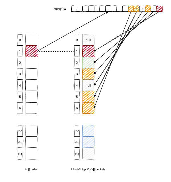
Let’s break down the logic using the diagram above:
buckets[2]was not originally hashed to index1, so the second bit ofradar[1]remains0.buckets[3],buckets[5], andbuckets[6]all have a base index of1. Consequently, we set the corresponding bits inradar[1]to1.
Insertion Logic
When inserting an element, we keep track of how far we have “probed” from the base index. If we find a slot within the 32-bit window, we update the radar bitmask.
protected V put(K key, V value, int hash) {
    // Increase the capacity if the threshold is met
    if (shouldGrow()) {
        grow();
    }

    int base = hash & (buckets.length - 1);
    int idx = base;
    int probing = 0;

    while(true) {
        // If we exceed the 32-slot radar window, we are forced to resize
        if (probing == 32) {
            grow();
            return put(key, value, hash);
        }

        if (buckets[idx] == null) {
            // It's a free spot
            buckets[idx] = new LProbEntry(key, value, hash);
            // Mark the bit in the radar entry for the base slot
            radar[base] |= (1 << probing);
            size++;
            return null;
        }
        else if (buckets[idx].key == null) {
            // It's a tombstone: reclaim the spot
            buckets[idx].key = key;
            buckets[idx].val = value;
            buckets[idx].hash = hash;
            radar[base] |= (1 << probing);
            size++;
            tombstones--;
            return null;
        }
        else if (buckets[idx].hash == hash && key.equals(buckets[idx].key)) {
            // Key match: perform an update
            V ret = buckets[idx].val;
            buckets[idx].val = value;
            return ret;
        }

        probing++;
        idx = (idx + 1) & (buckets.length - 1);
    }
}
Retrieval Logic
The advantage of the radar is that we can skip the equals() check and the hash check for any slot where the radar bit is 0. We would only examine “relevant” buckets that we know belong to this specific base index.
public V get(Object key) {
    if (null == key) {
        throw new IllegalArgumentException("Map doesn't support null keys");
    }

    int hash = hash(key);
    int idx = hash & (buckets.length - 1);
    int rd = radar[idx];

    // Quick exit: if the radar is 0, no elements with this base index exist
    if (rd == 0) {
        return null;
    }

    for(int bit = 0; bit < 32; bit++) {
        // Only check the bucket if the radar bit indicates a match resides here
        if (((rd >> bit) & 1) == 1) {
            if (buckets[idx].hash == hash && key.equals(buckets[idx].key)) {
                return buckets[idx].val;
            }
        }
        idx = (idx + 1) & (buckets.length - 1);
    }
    return null;
}
Analysis and Risks
To be honest, this specific implementation has some significant drawbacks:
- Checking the bit
((rd >> bit) & 1) == 1isn’t necessarily faster than simply checking ifbuckets[idx] == null, especially given modern CPU branch prediction and the overhead of bitwise shifts in a loop; - Enforcing a hard limit of 32 for the probing distance is a dangerous approach. If a user provides a poor
hashCode()implementation that causes a massive cluster, the map will trigger a resize every time a 33rd collision occurs. This could lead to a massive, sparse array that eventually crashes the JVM with anOutOfMemoryError(OOM).
Nevertheless, it was a fun exercise in metadata-assisted probing.
RobinHoodMap<K, V>
The RobinHoodMap<K, V> is my final open-addressing implementation, utilizing the Robin Hood hashing technique. This algorithm is a variation of linear probing that aims to reduce the variance of “distance from home” for all entries in the table.
For the full source code, please check this link.
The “Rich” and the “Poor”
In standard linear probing, an element that arrives late to a crowded neighborhood might be pushed very far from its base slot, leading to long search times. Robin Hood hashing fixes this by “taking from the rich and giving to the poor.”
In this context, an entry is “rich” if it is located close to its base slot (low distance) and “poor” if it has been pushed far away (high distance). During insertion, if a new entry is “poorer” than the one currently occupying a slot, they swap places.
To implement this, we add a dist attribute to our entry class:
public static class Entry<K, V> implements Map.Entry<K, V> {
    private K key;
    private V value;
    private int hash;
    private int dist; // Distance from the base slot

    // (more code)
}
Let’s look at how an insertion works with the following visual example:
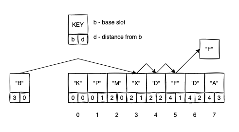
- We want to insert
"B". Its base slot is3. - We check index
3. It’s occupied byX. Sincedistance(B,3) == 0is not greater thandistance(X, base(X)), we move to the next slot. - We check index
4. It’s occupied byD. Sincedistance(B,3) == 1is not greater thandistance(D, base(D)), we move to the next slot. - We check index
5. It’s occupied byF. Here,distance(B,3) == 2, whileFis only1slot away from its own base. BecauseBis poorer thanF, we swap them. - We now continue the process, but this time trying to find a new home for the displaced
F.
Implementation of put
While get and remove remain largely the same as in LProbMap, the put operation is where the “Robin Hood” logic lives:
protected V put(K key, V value, int hash) {
    if (null == key) {
        throw new IllegalArgumentException("Map doesn't support null keys");
    }
    increaseCapacity();

    K cKey = key;
    V cVal = value;
    int cHash = hash;
    int cDist = 0; // Current distance from base
    V oldVal = null;

    int idx = hash & (buckets.length - 1);

    while (true) {
        // If the slot is empty, we simply insert the element
        if (null == buckets[idx]) {
            buckets[idx] = new Entry<>(cKey, cVal, cHash, cDist);
            this.size++;
            break;
        }
        // If we found the key, update the value
        else if (cHash == buckets[idx].hash && cKey.equals(buckets[idx].key)) {
            oldVal = buckets[idx].value;
            buckets[idx].value = cVal;
            // No swap needed, we just break
            break;
        }
        // ROBIN HOOD SWAP: If current entry is "poorer" than the occupant
        else if (cDist > buckets[idx].dist) {
            // Swap current element with the occupant
            K tmpKey = buckets[idx].key;
            V tmpVal = buckets[idx].value;
            int tmpHash = buckets[idx].hash;
            int tmpDist = buckets[idx].dist;

            buckets[idx].key = cKey;
            buckets[idx].value = cVal;
            buckets[idx].hash = cHash;
            buckets[idx].dist = cDist;

            // Now we look for a home for the displaced element
            cKey = tmpKey;
            cVal = tmpVal;
            cHash = tmpHash;
            cDist = tmpDist;
        }

        // Standard linear probing to the next slot
        cDist++;
        idx = (idx + 1) & (buckets.length - 1);
    }
    return oldVal;
}
Why use Robin Hood Hashing?
The primary advantage of this technique is that it significantly reduces the variance of the distance entries travel from their base slots.
In a standard linear probing table, you might have one unlucky element that is 50 slots away from home, making its retrieval very slow. In a Robin Hood table, that “cost” is shared across the neighborhood.
This leads to much more consistent search times and helps prevent the “long tail” of performance degradation during high load factors.
Benchmarks
After implementing the six Open Addressing maps: LProbMap.java, LProbBinsMap.java, LProbRadarMap.java, PerturbMap.java, RobinHoodMap.java, and the SoA variant, it was time to put them to the test against the standard HashMap<K,V> reference.
Microbenchmarking in Java is notoriously difficult due to JIT optimizations and JVM warmups. To handle this properly, I used JMH combined with MockNeat for data generation.
The benchmarks are available in the repository under the performance/jmh folder. To run them yourself, refer to the Main.class:
// Cleans the existing generated data from previous runs
InputDataUtils.cleanBenchDataFolder();

Options options = new OptionsBuilder()
        // Benchmarks to include
        .include(RandomStringsReads.class.getName())
        .include(SequencedStringReads.class.getName())
        .include(AlphaNumericCodesReads.class.getName())
        // Configuration
        .timeUnit(TimeUnit.MICROSECONDS)
        .shouldDoGC(true)
        .resultFormat(ResultFormatType.JSON)
        .addProfiler(GCProfiler.class)
        .result("benchmarks_" + System.currentTimeMillis() + ".json")
        .build();

new Runner(options).run();
The execution generates a JSON result file which can be visualized using JMH Visualizer or a custom Python script.
Benchmark Configuration
I defined three primary benchmark scenarios: RandomStringsReads, SequencedStringReads, and AlphaNumericCodesReads. They share the following configuration:
@BenchmarkMode(Mode.AverageTime)
@OutputTimeUnit(TimeUnit.MICROSECONDS)
@State(Scope.Benchmark)
@Fork(value = 3, jvmArgs = {"-Xms6G", "-Xmx16G"})
@Warmup(iterations = 2, time = 5)
@Measurement(iterations = 4, time = 5)
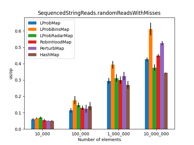
Each class tests two specific behaviors: randomReads() (where keys are guaranteed to exist) and randomReadsWithMisses() (where there is a 50% chance the key is missing).
@Benchmark
@CompilerControl(CompilerControl.Mode.INLINE)
public void randomReads(Blackhole bh) {
    bh.consume(testedMap.get(fromStrings(keys).get()));
}
Data Generation Strategies
1. RandomStringsReads
Keys are generated using MockNeat’s probabilities() method to simulate diverse real-world data:
- 20% Full Names
- 20% Addresses
- 20% Dictionary Words
- 20% Car Make/Models
- 20% String-encoded Integers
2. SequencedStringsReads
Uses intSeq().mapToString() to generate keys like "0", "1", "2". This tests how the maps handle inputs with high mathematical patterns.
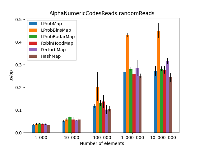
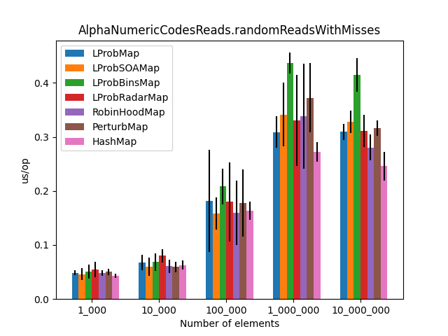
3. AlphaNumericCodesReads
Uses strings().size(6).type(StringType.ALPHA_NUMERIC) to generate short, fixed-length codes.
The Results
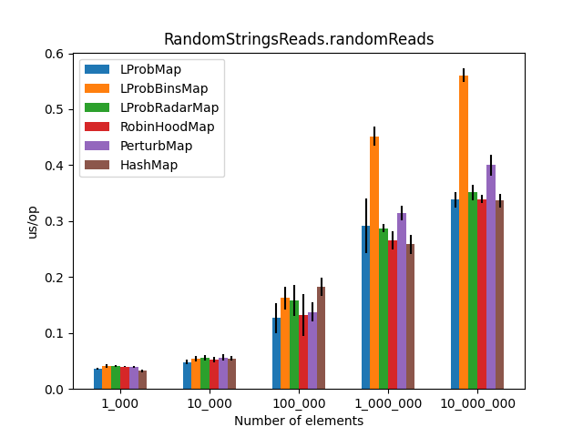
After approximately 6 hours of execution, the initial results were plotted. The charts compare average time (lower is better) across increasing map sizes (from 1,000 to 10,000,000 entries).
| Random Reads | Reads with Misses |
|---|---|
 |  |
 |  |
 |  |
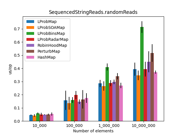
Including LProbSOAMap<K,V>
After dzaima’s SoA (Structure of Arrays) contribution, I re-ran the suite. The SoA variant significantly improved performance by reducing object overhead.
| Random Reads (with SoA) | Reads with Misses (with SoA) |
|---|---|
 |  |
 |  |
 |  |
Wrapping Up
This project was both a fun and frustrating dive into the “other half” of Java performance (he JIT compiler). Here are my main takeaways:
- The JIT Factor: In Java, you are only “half-smart.” You can write optimized code, but you have no direct control over inlining or the final machine code produced by the JIT.
- Performance:
LProbMapandRobinHoodMapperformed surprisingly well againstHashMapfor datasets under 1 million entries.LProbSOAMapwas the standout performer, outshiningHashMapuntil the size exceeded 10 million entries, at which pointHashMap’s chaining optimizations began to dominate. - The “Bins” Mystery: I had high hopes for
LProbBinsMap, but it performed the worst. The extra indirection likely caused too many cache misses in the JVM environment. - Should you use these? Probably not.
HashMap<K,V>is battle-tested, bullet-proof, and highly optimized for the general case.
If you have ideas for further optimizations (like shifting elements instead of using tombstones) the repository is open for PRs.
Discussion
Source Code & Contributions
Spot an error or have an improvement? Open a PR directly for this article .