Implementing Hash Tables in C
Table of contents
Code
If you want to skip the theory and dive straight into the implementation, you can find the source code here:
- Separate Chaining:
git clone git@github.com:nomemory/chained-hash-table-c.git - Open Addressing:
git clone git@github.com:nomemory/open-adressing-hash-table-c.git
Note: The code is written in C and needs to be compiled with the
-std=c99flag.
Introduction
Outside the domain of computers, the word hash means to chop or mix something.
In Computer Science, a hash table is a fundamental data structure that maps a set of keys to a set of values. Each pair <key, value> is known as an entry. The beauty of a hash table is that given a key, you can retrieve its corresponding value almost instantly. You can also add or remove these pairs as needed.
Clarification: A hash table should not be confused with hash trees or hash lists.
In some ways, a hash table acts like a supercharged array. Consider this standard C array:
int arr[] = {100, 200, 300};
printf("%d\n", arr[1]); // Output: 200
When we write arr[1], we are “peeping” at the value associated with index 1. In our case, that value is 200. A hash table works on a similar principle, but with a significant twist: the key can be anything (a string, a large number, or even a custom object) not just a sequential numerical index.
Most modern programming languages provide a built-in hash table implementation. The terminology varies, but the underlying mechanics remain consistent:
- C++:
std::unordered_map - Java:
HashMap - Python:
dict(Dictionary)
Let’s look at how we store and retrieve a hex color value using the key "RED" across these languages:
C++ (unordered_map)
#include <iostream>
#include <string>
#include <unordered_map>

int main() {
    std::unordered_map<std::string, std::string> colors = {
        {"RED", "#FF0000"},
        {"GREEN", "#00FF00"},
        {"BLUE", "#0000FF"}
    };
    std::cout << colors["RED"] << std::endl;
}
Java (HashMap)
import java.util.HashMap;

public class HashMapExample {
    public static void main(String[] args) {
        HashMap<String, String> colors = new HashMap<>();
        colors.put("RED", "#FF0000");
        colors.put("GREEN", "#00FF00");
        colors.put("BLUE", "#0000FF");

        System.out.println(colors.get("RED"));
    }
}
Python (dict)
colors = {
    "RED": "#FF0000",
    "GREEN": "#00FF00",
    "BLUE": "#0000FF"
}
print(colors["RED"])
Regardless of the syntax, the result is the same: "#FF0000".
Performance: Why Size Doesn’t Matter
The most impressive feature of hash tables is their efficiency. For most operations, they offer constant time complexity ($O(1)$). This means that searching for an element takes the same amount of time whether you have 10 entries or 10 million entries.
In a Binary Search Tree, searching is $O(\log n)$; as the tree grows, $n$ increases, and searching for an element takes more time. But with a properly tuned hash table, you have near-instant access to your data regardless of how much it scales.
| Operation | Average Time Complexity | Worst-case Complexity |
|---|---|---|
| Search (Get) | $O(1)$ | $O(n)$ |
| Insert (Add) | $O(1)$ | $O(n)$ |
| Update | $O(1)$ | $O(n)$ |
| Delete (Remove) | $O(1)$ | $O(n)$ |
This remarkable performance is powered by clever mathematical algorithms called hash functions. They are the “engine” behind the scenes, transforming arbitrary keys into specific array indices.
Before we jump into the C implementation, we need to take a short mathematical detour into the wonderful world of hash functions. They are often less intimidating than they look on the surface.
Hash Functions
In plain English, a hash function is a mathematical tool that “chops” or maps data of arbitrary size to a fixed size.
From a mathematical perspective, a hash function is a function $H : X \rightarrow [0, M)$ that takes an element $x \in X$ and associates it with a positive integer $H(x) = m$, where $m \in [0, M)$.
In this definition:
- $X$ represents the Keyspace (the set of all possible inputs, which can be bounded or unbounded).
- $M$ is the Table Size, a positive finite number ($0 < M < \infty$) representing the number of available slots in our table.
Let’s take a look at the following example:

In the diagram above, Paris, Berlin, Warsaw, Bucharest, and Athens are elements of $X$. If $X$ is the set of all European Capitals, then the size of the set, $n(X)$, is 48.
Our hashing function $H : X \rightarrow [0, 16)$ maps these strings to integers:
H("Paris")returns00H("Berlin")returns01H("Warsaw")returns04H("Bucharest")returns03H("Athens")returns04
Since there are 48 capitals but only 16 possible slots ($48 > 16$), no matter how we write $H$, some cities will inevitably share the same index $m$. In our hypothetical example, this happens with H("Warsaw") = H("Athens") = 4.
Hash Collisions
Whenever two distinct elements $x_{1}, x_{2} \in X$ result in $H(x_{1}) = H(x_{2}) = m_{x}$, we have a hash collision.
In our example, we have a collision for $x_{1} = \text{Warsaw}$ and $x_{2} = \text{Athens}$ because both map to index 4.
Collisions are not “game-breaking” per-se, as long as $n(X) > M$, they are a mathematical certainty (the Pigeonhole Principle). However, a good hash function creates significantly fewer collisions than a bad one.
The absolute worst hash function we could write is a constant function: $H(x) = c$. In this case, every single element collides at the same index, effectively turning our hash table into a very slow linked list.
Another pitfall is choosing a function that is not deterministic. $H(x)$ must always return the same result for the same $x$, regardless of external factors like time or memory state.
Cryptographic vs. Non-Cryptographic: Cryptographic hash functions are a specialized family designed for security. They must be resistant to preimage attacks and collisions. The functions used in hash table implementations are significantly “less pretentious”, we prioritize raw speed over security.
What makes a “Good” Hash Function?
Picking a hash function is a mix of statistics, number theory, and empiricism. Generally, we look for these three pillars:
- Low Collision Rate: It should minimize the number of keys mapping to the same index.
- Uniform Distribution: It should disperse hashes evenly across the $[0, M)$ interval to avoid “clumping.”
- Efficiency: Computation should be fast, ideally approaching $O(1)$.
Families of Hashing Functions
We can categorize these functions into several common families:
- Division Hashing: Using the remainder of division (mod).
- Multiplicative Hashing: Using fractional parts and bit-shifts (multiplicative).
- Bit-shift/Mixing: Scrambling bits to ensure small changes in input create large changes in output.
The advanced math behind these functions is vast. While PhD papers are written on finding the most efficient way to “mix” bits, as engineers, we can keep things pragmatic by focusing on a few proven implementations.
Division hashing
The simplest hash function we can write uses the modulo % operation, and it’s aptly called division hashing.
It works on positive integers, so let’s suppose we can represent our initial input data $x_{1}, x_{2}, … x_{n} \in X \subset \mathbb{N}$ as non-negative integers.
The formula for our hash function is $H_{division}(x) = x \mod M$, where $H_{division} : X \rightarrow [0, M)$. In plain English, this means the hash of a given value $x$ is the remainder of $x$ divided by $M$.
Writing this in C is trivial:
uint32_t hashf_division(uint32_t x, uint32_t M) {
    return x % M;
}
On the surface, hashf_division() checks all the requirements for a good hashing function. It’s fast and easy to understand. It performs well as long as the input data is guaranteed to be perfectly random, without obvious numerical patterns.
Let’s test it with:
M=4;1,000,000uniformly distributed positive integers as input ($X$)
Logic suggests that the input will be evenly distributed between 4 hash values: 0, 1, 2, and 3. While collisions are inevitable (since our input set is 250,000 times larger than $M$), they should be balanced.
#include <stdio.h>
#include <stdlib.h>
#include <time.h>
#include <stdint.h>

#define M_VAL 4
#define X_VAL 1000000

uint32_t hashf_division(uint32_t x, uint32_t M) {
    return x % M;
}

int main() {
    srand(time(0));
    uint32_t i, hash;
    int buckets[M_VAL] = {0};

    for(i = 0; i < X_VAL; i++) {
        hash = hashf_division(rand(), M_VAL);
        buckets[hash]++;
    }

    for(i = 0; i < M_VAL; i++) {
        printf("bucket[%u] has %u elements\n", i, buckets[i]);
    }
    return 0;
}
A typical output might look like this:
bucket[0] has 250146 elements
bucket[1] has 249361 elements
bucket[2] has 250509 elements
bucket[3] has 249984 elements
The results are satisfactory: the input is evenly distributed, and the % operation is efficient. However, what happens if our data isn’t random? What if it follows an obvious pattern?
Let’s change the input to only even numbers:
hash = hashf_division(rand() & -2, M_VAL);
The output shifts dramatically:
bucket[0] has 500810 elements
bucket[1] has 0 elements
bucket[2] has 499190 elements
bucket[3] has 0 elements
Buckets 1 and 3 are completely empty. Mathematically, for $H(x) = x \mod 4$, if $x$ is even, the remainder can only be 0 or 2. This makes the function extremely sensitive to “input patterns.”
We can improve this by choosing $M$ to be a prime number. Changing M=4 to M=7 would yield a much more balanced distribution even with even-numbered inputs. In practice, certain primes work better than others:
To further optimize, Donald Knuth proposed $H_{division}^{Knuth}(x) = x(x + 3) \mod M$. Despite these tweaks, division hashing is less common in high-performance implementations because modulo operations are significantly more “expensive” in CPU cycles than multiplication or bit-shifting.
Note: We call the resulting hashes buckets. Once we start implementing the actual hash table, this terminology will become much clearer.
Multiplicative hashing
A more practical approach for generating uniform hash values is multiplicative hashing. Like division hashing, it works on positive integers.
The general formula is: $H_{multip}(x) = \lfloor M \cdot ( (A \cdot x) \mod 1 ) \rfloor$
However, in a computer with a word size $W$, we usually represent it as: $H_{multip}(x) = (A \cdot x \mod W) \gg (w - m)$
Where:
- $M = 2^m$ (total buckets)
- $W = 2^w$ (machine word size, e.g., $2^{32}$)
- $A$ is a constant multiplier.
By using bitwise operations, we can avoid the slow modulo. $A \cdot x \mod 2^w$ simply grabs the $w$ low-order bits. Shifting right by $(w-m)$ then isolates the most significant bits of that result.
In C, the raw version looks like this:
uint32_t hashf_multip(uint32_t x, uint32_t w, uint32_t m, uint32_t A)  {
    return (x * A) >> (w - m);
}
A mathematically “sweet” choice for $A$ is $A \approx \phi \cdot 2^w$, where $\phi$ is the golden ratio ($\approx 0.618$). This specific implementation is known as Fibonacci hashing.
Depending on your word size, $A$ should be:
| $w$ | $A = 2^w \cdot \phi \approx$ |
|---|---|
| 16 | 40,503 |
| 32 | 2,654,435,769 |
| 64 | 11,400,714,819,323,198,485 |
We can now simplify our C function using constants:
#define HASH_A (uint32_t)2654435769
#define HASH_W 32
#define HASH_M 3 // For 2^3 = 8 buckets

uint32_t hashf_multip(uint32_t x) {
    return (x * HASH_A) >> (HASH_W - HASH_M);
}
As noted in various technical analyses, Fibonacci hashing can have issues where higher-value bits don’t influence lower-value bits enough. We can fix this with a bit of “mixing” (XORing) before the multiplication:
uint32_t hashf_multip_mixed(uint32_t x) {
    x ^= x >> (HASH_W - HASH_M);
    return (x * HASH_A) >> (HASH_W - HASH_M);
}
This version provides better diffusion at the minor cost of a few extra CPU cycles.
Hashing strings
Converting non-numerical data like strings into positive integers (uint32_t) is fundamentally a process of processing a sequence of bits. Since every character has a numerical ASCII/UTF-8 value, we can iterate through the string to compute a final hash.
In the K&R Book (1st ed), a simple, but ultimately ineffective, algorithm was proposed: What if we simply sum the numerical values of all characters in the string?
uint32_t hashf_krlose(char *str) {
    uint32_t hash = 0;
    char c;
    while((c=*str++)) {
        hash += c;
    }
    return hash;
}
Unfortunately, hashf_krlose is “extremely” sensitive to input patterns. Because addition is commutative, any permutation of the same characters (anagrams) will result in the same hash. It is easy to apply a little Gematria to create inputs that repeatedly return identical hashes.
For example:
char* input[] = { "IJK", "HJL", "GJM", "FJN" };
uint32_t i;
for(i = 0; i < 4; i++) {
    printf("%u\n", hashf_krlose(input[i]));
}
The hash values for "IJK", "HJL", "GJM", and "FJN" are all 222.
While replacing += (summing) with ^= (XORing) might feel like an improvement, patterns that break the function are still trivial to create. The order of characters must matter for the hash to be effective.
The Rolling Hash Template
The most common “good” hash functions for strings follow a specific multiplicative template:
#define INIT <some_value>
#define MULTIP <some_value>

uint32_t hashf_generic(char* str) {
    uint32_t hash = INIT;
    char c;
    while((c = *str++)) {
        hash = MULTIP * hash + c;
    }
    return hash;
}
djb2
When INIT = 5381 and MULTIP = 33, the function is known as the Bernstein hash djb2 (dating back to 1991). It is remarkably effective at distributing strings uniformly.
Implementing it in C is straightforward:
#define INIT 5381
#define MULT 33

uint32_t hashf_djb2_m(char *str) {
    uint32_t hash = INIT;
    char c;
    while((c = *str++)) {
        hash = hash * MULT + c;
    }
    return hash;
}
You will often see a version of djb2 that uses a clever bit-shifting trick:
#define INIT 5381

uint32_t hashf_djb2(char *str) {
    uint32_t hash = INIT;
    char c;
    while((c = *str++)) {
        // Equivalent to: hash * 33 + c
        hash = ((hash << 5) + hash) + c;
    }
    return hash;
}
The expression (hash << 5) + hash is equivalent to hash * 32 + hash, which equals hash * 33. Historically, CPUs performed bitshifts and additions much faster than multiplications. While modern compilers usually optimize this automatically, this idiom remains a classic in the C community.
sdbm
The sdbm algorithm was created for the sdbm database library (a public-domain re-implementation of ndbm). It is excellent at scrambling bits to create a high-distribution hash.
uint32_t hashf_sdbm(char *str) {
    uint32_t hash = 0;
    char c;
    while((c = *str++)) {
        // A complex mix of bit shifts
        hash = c + (hash << 6) + (hash << 16) - hash;
    }
    return hash;
}
Reducing collisions: Finalizers
Even a good string hash can be improved using a finalizer. A finalizer is an additional set of bitwise operations applied to the result of a hash function to ensure that even small differences in the input are reflected in the final output bits (improving “avalanche” properties).
A common finalizer found in MurmurHash is fmix32:
uint32_t ch_hash_fmix32(uint32_t h) {
    h ^= h >> 16;
    h *= 0x3243f6a9U;
    h ^= h >> 16;
    h *= 0xabcd1234U; // Additional mixing constant
    h ^= h >> 16;
    return h;
}
Applying this to the output of djb2 or sdbm can significantly harden the distribution:
uint32_t final_hash = ch_hash_fmix32(hashf_sdbm("some string"));
More exploration
We have only scratched the surface. Choosing the “best” hash is often a trade-off between computation speed and collision resistance.
- FNV-1a - Excellent for small strings; very fast.
- SipHash - Designed to be cryptographically secure against “hash flooding” attacks; used as the default in many modern languages (Rust, Python, Ruby).
- MurmurHash3 - The gold standard for general-purpose non-cryptographic hashing.
- Zobrist Hashing - Specifically used for board game positions (Chess/Go) to identify previously analyzed states.
For most day-to-day C engineering, a robust implementation of djb2 or FNV-1a with a good finalizer is more than sufficient. Simple is usually better.
Implementing Hash Tables
Hash tables are fundamental data structures that associate a set of keys with a set of values. Each <key, value> pair is an entry in the table. By knowing the key, we can look for its corresponding value (GET), add new entries (PUT), or remove existing ones (DEL).
In a hash table, data is stored in an array where each pair has its own index (or bucket). Accessing this data is highly efficient because, in an ideal scenario, we can jump directly to the required memory address.
The specific bucket is computed by applying a hash function to a key:
$$hash_{function}(key) \rightarrow \text{bucket index}$$Because multiple keys can hash to the same index (a “collision”), we must decide how to handle these overlaps. The primary strategies are:
1. Separate Chaining
This approach treats each bucket as the head of a secondary data structure.
- Linked Lists: The most common form. Each bucket references a linked list. If a collision occurs, the new entry is simply appended to the list at that index. GET operations require traversing the list to find the exact key.
- Dynamic Arrays: Instead of a list, each bucket is a dynamically resizing array. This improves cache locality but makes resizing more expensive.
- Red-Black Trees: Used as an optimization (notably in Java 8+
HashMap). If a bucket’s list grows beyond a certain threshold, it “morphs” into a balanced tree to ensure $O(\log n)$ worst-case search time.
2. Open Addressing
There are no secondary structures; every <key, value> pair lives directly in the main array.
- If a collision occurs, the algorithm uses Probing to find the next available empty slot.
- The simplest method is Linear Probing: if index $i$ is full, try $i+1$, then $i+2$, and so on.
- While Open Addressing is more complex to implement (especially deletion, which requires “tombstones”), it is extremely cache-friendly because all data resides in a contiguous block of memory.
Separate Chaining (using Linked Lists)
To better understand how Separate Chaining works, let’s look at a hash table associating European capitals (keys) with their corresponding countries (values):
| European Capital (Key) | European Country (Value) |
|---|---|
| “Paris” | “France” |
| “Berlin” | “Germany” |
| “Warsaw” | “Poland” |
| “Bucharest” | “Romania” |
| “Athens” | “Greece” |
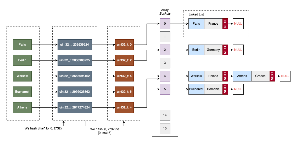
The Multi-Step Hashing Process
Since our keys and values are strings (char*), we must perform two distinct “mapping” steps to find the correct bucket:
- Hash Code Generation: We reduce the complex key (the string) to a 32-bit unsigned integer (
uint32_t). A popular choice for strings is the djb2 algorithm. This step belongs to the “data type” logic, the hash table itself shouldn’t need to know how to “read” every possible data format. - Bucket Compression: We take that large
uint32_tand map it to the range $[0, M)$, where $M$ is our array size. We typically use division hashing ($hash \pmod M$) or multiplicative hashing for this.
Once the bucket index is determined:
- If the bucket is empty (
NULL), we allocate a new node and place it there. - If a node already exists, we have a collision. we append the new node to the chain (linked list). If the key is already present in that chain, we simply update the existing value to keep the map unique.
A Generic Implementation
Ideally, our hash table should be as generic as possible so it can be reused for various key/value combinations. Writing a new implementation every time your data type changes is inefficient and violates the DRY (Don’t Repeat Yourself) principle.
The bad news: C is not exactly known for being a generic-friendly language. Unlike C++ with its templates or Java with Generics, C requires a bit of manual labor to handle multiple types.
The good news: C is flexible enough to make generic programming happen through two main patterns:
- Using
void*: The “generic pointer” allows us to pass around addresses to any data type. - Using
#macros: The preprocessor can generate specialized code for specific types at compile-time, essentially a poor man’s version of C++ templates.
Inspiration: I recently discovered a library called STC that uses a clever macro-based approach for generic data structures in C. It’s well worth a look if you want to see how far you can push the preprocessor.
While I generally prefer the performance and type-safety of #macros for production, they are a nightmare for tutorials. Macros become messy quickly, obfuscate errors, and make code difficult to debug. Therefore, for this implementation, we will use void* to handle generic data. This keeps the logic clean and the focus on the data structure itself rather than preprocessor wizardry.
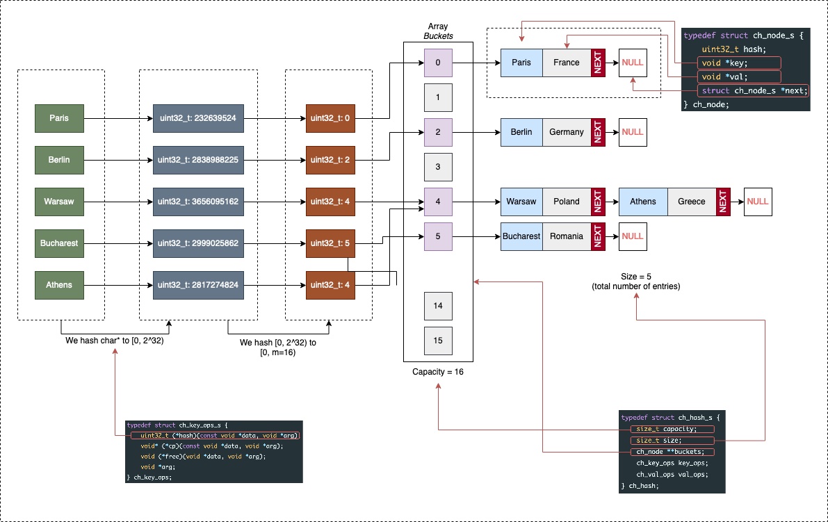
The Model
We begin by defining the structures (struct) that form the skeleton of our hash table. The core structure, ch_hash, acts as the manager of the entire table:
capacity: The total number of available buckets (the size of the array).size: The total number of elements currently stored in the table.buckets: A pointer to an array of linked list heads.key_opsandval_ops: Functional “traits” that tell the hash table how to handle the specific data types you choose to store.
typedef struct ch_hash_s {
    size_t capacity;
    size_t size;
    ch_node **buckets;
    ch_key_ops key_ops;
    ch_val_ops val_ops;
} ch_hash;
Since we are using Separate Chaining, each bucket is the head of a linked list composed of nodes:
typedef struct ch_node_s {
    uint32_t hash;
    void *key;
    void *val;
    struct ch_node_s *next;
} ch_node;
The ch_node structure is our data container:
uint32_t hash: This is the pre-computed hash value of the key. We store it so that when we need to rehash (resize) the table, we don’t have to run the expensive hashing function again for every single element.keyandval: These arevoid*pointers. This is the C way of saying “I can point to anything.” It gives us the flexibility to store strings, integers, or custom structs.next: A pointer to the next node in the chain, resolving collisions by linking elements that map to the same bucket.
Data-Specific Operations: The Contract
The “unknown” members, ch_key_ops and ch_val_ops, are where the magic of generic programming in C happens. Because the hash table only sees void*, it doesn’t know how to compare two keys, how to copy them, or even how to free their memory. We must provide those instructions:
typedef struct ch_key_ops_s {
    uint32_t (*hash)(const void *data, void *arg);
    void* (*cp)(const void *data, void *arg);
    void (*free)(void *data, void *arg);
    bool (*eq)(const void *data1, const void *data2, void *arg);
    void *arg;
} ch_key_ops;

typedef struct ch_val_ops_s {
    void* (*cp)(const void *data, void *arg);
    void (*free)(void *data, void *arg);
    bool (*eq)(const void *data1, const void *data2, void *arg);
    void *arg;
} ch_val_ops;
These structures use function pointers to create a contract. You are essentially telling the hash table: “I want to use strings as keys; here is the specific function to hash a string, the function to compare two strings, and the function to clean them up.”
If function pointers feel a bit like “black magic,” think of them as variables that hold the address of a function instead of a number. This allows us to pass behavior as an argument.
Implementation Example: Strings
To use strings (char*) in our table, we implement the functions defined in our “ops” contract. Note that since we use void*, we must manually cast the pointers back to char* inside each function.
// A finalizer to improve hash distribution (MurmurHash3 mixer)
static uint32_t ch_hash_fmix32(uint32_t h) {
    h ^= h >> 16;
    h *= 0x3243f6a9U;
    h ^= h >> 16;
    return h;
}

// Hashing: Using djb2 for string data
uint32_t ch_string_hash(const void *data, void *arg) {
    uint32_t hash = 5381;
    const char *str = (const char*) data;
    char c;
    while((c = *str++)) {
        hash = ((hash << 5) + hash) + c; // hash * 33 + c
    }
    return ch_hash_fmix32(hash);
}

// Deep Copy: Duplicating the string in memory
void* ch_string_cp(const void *data, void *arg) {
    const char *input = (const char*) data;
    char *result = malloc(strlen(input) + 1);
    if (!result) {
        fprintf(stderr, "malloc() failed\n");
        exit(EXIT_FAILURE);
    }
    strcpy(result, input);
    return result;
}

// Equality: Comparing string contents
bool ch_string_eq(const void *data1, const void *data2, void *arg) {
    return strcmp((const char*)data1, (const char*)data2) == 0;
}

// Memory Cleanup
void ch_string_free(void *data, void *arg) {
    free(data);
}
Finally, we bundle these functions into instances that our hash table can use:
ch_key_ops ch_key_ops_string = { ch_string_hash, ch_string_cp, ch_string_free, ch_string_eq, NULL };
ch_val_ops ch_val_ops_string = { ch_string_cp, ch_string_free, ch_string_eq, NULL };
By separating the logic of how to store (the hash table) from the logic of what is stored (the traits), we’ve built a structure that can handle almost any data type with minimal code changes.
Now, let’s see how these structures fit together in memory:
The Interface
Our hash table (ch_hash) will support and publicly expose the following functions (interface):
// Creates a new hash table
ch_hash *ch_hash_new(ch_key_ops k_ops, ch_val_ops v_ops);

// Free the memory associated with the hash (and all of its contents)
void ch_hash_free(ch_hash *hash);

// Gets the value corresponding to a key
// If the key is not found returns NULL
void* ch_hash_get(ch_hash *hash, const void *k);

// Checks if a key exists or not in the hash table
bool ch_hash_contains(ch_hash *hash, const void *k);

// Adds a <key, value> pair to the table
void ch_hash_put(ch_hash *hash, const void *k, const void *v);

// Prints the contents of the hash table
void ch_hash_print(ch_hash *hash, void (*print_key)(const void *k), void (*print_val)(const void *v));

// Get the total number of collisions
uint32_t ch_hash_numcol(ch_hash *hash);
As you might’ve noticed, there’s no function for deleting an entry. That’s intentionally left out as a proposed exercise.
Before implementing the enumerated methods, it’s good to clarify a few things that are not obvious from the interface itself.
Dynamic Resizing and Rehashing
Just for fun (best practices are fun!), our hash table will grow automatically if its size reaches a certain threshold. Every time we insert a new element, we check if the threshold has been reached and if it’s time to increase the capacity (and the number of available buckets).
When resizing occurs, a rehashing of everything is performed, old entries are mapped to new buckets based on the new capacity. We define the following constants to control this (which can be tweaked later):
#define CH_HASH_CAPACITY_INIT (32)
#define CH_HASH_CAPACITY_MULT (2)
#define CH_HASH_GROWTH (1)
And then perform the following check each time we insert a new item:
// Grow if needed
if (hash->size > hash->capacity * CH_HASH_GROWTH) {
    ch_hash_grow(hash);
        // -> The function will perform a full rehashing to a new array of buckets
        // of size [hash->capacity * CH_HASH_CAPACITY_MULT]
}
The ch_hash_grow(ch_hash *hash) function is not defined as part of the interface; it’s private. We won’t be exposing it to the header file.
Internal Node Retrieval
Another function not exposed in our public interface is ch_node* ch_hash_get_node(ch_hash*, const void*). This is used internally to check if a node exists. If it does, it retrieves the entire node; otherwise, it returns NULL.
The reason we have two functions for retrieving data is simple:
void* ch_hash_get(ch_hash *hash, const void *k);(public) - Returns only the value to the user.ch_node* ch_hash_get_node(ch_hash *hash, const void *key)(private) - Works on the internalch_nodestructure used by our implementation.
By separating these, we keep the internal “plumbing” of the linked lists hidden from the user, providing a cleaner and more secure API.
Creating/Destroying a hash table
Memory management is the most critical part of C development. To handle our ch_hash structure, we implement two primary functions: ch_hash_new (the constructor) and ch_hash_free (the destructor).
ch_hash_new dynamically allocates memory for the main hash structure and its initial array of buckets. We initialize the capacity and set all buckets to NULL to indicate they are currently empty.
ch_hash *ch_hash_new(ch_key_ops k_ops, ch_val_ops v_ops) {
    ch_hash *hash;

    hash = malloc(sizeof(*hash));
    if(NULL == hash) {
        fprintf(stderr, "malloc() failed in file %s at line # %d\n", __FILE__, __LINE__);
        exit(EXIT_FAILURE);
    }

    hash->size = 0;
    hash->capacity = CH_HASH_CAPACITY_INIT;
    hash->key_ops = k_ops;
    hash->val_ops = v_ops;

    // Allocate the array of bucket pointers
    hash->buckets = malloc(hash->capacity * sizeof(*(hash->buckets)));
    if (NULL == hash->buckets) {
        fprintf(stderr, "malloc() failed in file %s at line # %d\n", __FILE__, __LINE__);
        free(hash); // Clean up the structure before exiting
        exit(EXIT_FAILURE);
    }

    for(int i = 0; i < hash->capacity; i++) {
        hash->buckets[i] = NULL;
    }

    return hash;
}
A Note on Best Practices: Using
exit(EXIT_FAILURE);within a library is generally discouraged. It abruptly terminates the host program, preventing it from performing its own cleanup. In a production-grade library, it is better to returnNULLand let the caller handle the error.
ch_hash_free is responsible for a “deep” de-allocation. It doesn’t just free the main structure; it must traverse every bucket and follow every linked list to free the nodes.
void ch_hash_free(ch_hash *hash) {
    ch_node *crt;
    ch_node *next;

    for(int i = 0; i < hash->capacity; ++i) {
        crt = hash->buckets[i];
        while(NULL != crt) {
            next = crt->next;

            // Delegate memory cleanup to the data-specific traits
            hash->key_ops.free(crt->key, hash->key_ops.arg);
            hash->val_ops.free(crt->val, hash->val_ops.arg);

            // Free the container node
            free(crt);
            crt = next;
        }
    }
    // Free the buckets array and finally the hash structure itself
    free(hash->buckets);
    free(hash);
}
The logic in ch_hash_free is straightforward except for the specific cleanup of keys and values:
hash->key_ops.free(crt->key, hash->key_ops.arg);
hash->val_ops.free(crt->val, hash->val_ops.arg);
Since the hash table stores generic data via void*, it has no inherent knowledge of how to destroy that data (e.g., should it call free(), or is it a complex struct requiring its own destructor?). By using the free function pointers referenced inside key_ops and val_ops, the table maintains its generic nature while ensuring no memory leaks occur.
Retrieving a value from the hash table
To find an entry in our table, we need a way to map our uint32_t hash back into the range of our available buckets: $[0, \text{hash->capacity})$. For the sake of simplicity, we will use the modulo operator %, implementing the division hashing method discussed earlier.
The core retrieval logic is handled by a private helper function, ch_hash_get_node. This function is responsible for the heavy lifting: calculating the index and traversing the potential collision chain.
static ch_node* ch_hash_get_node(ch_hash *hash, const void *key) {
    ch_node *result = NULL;
    ch_node *crt = NULL;
    uint32_t h;
    size_t bucket_idx;

    // 1. Compute the hash of the key using the data-specific trait
    h = hash->key_ops.hash(key, hash->key_ops.arg);

    // 2. Determine the bucket index using division hashing
    bucket_idx = h % hash->capacity;
    crt = hash->buckets[bucket_idx];

    // 3. Traverse the linked list (collision chain) at this bucket
    while(NULL != crt) {
        // We first compare hashes for speed; if they match, we perform
        // a "deep" equality check using the trait provided by the user.
        if (crt->hash == h && hash->key_ops.eq(crt->key, key, hash->key_ops.arg)) {
            result = crt;
            break;
        }
        crt = crt->next;
    }

    // Returns the node if found, otherwise NULL
    return result;
}
By storing the uint32_t hash directly within each ch_node, we gain a significant performance optimization. Calling the eq function pointer (which might involve an expensive strcmp) is only necessary if the integer hashes match first.
Finally, we expose the public ch_hash_get function. This is a thin wrapper designed to “filter” the results, returning only the user’s data (void*) rather than our internal node structure.
void* ch_hash_get(ch_hash *hash, const void *k) {
    ch_node *result = NULL;
    if (NULL != (result = ch_hash_get_node(hash, k))) {
        return result->val;
    }
    return NULL;
}
Adding an entry to the hash table
The ch_hash_put method is the workhorse of our implementation. It is responsible for inserting new <key, value> pairs or updating existing ones.
The logic follows a clear path:
- Check Existence: We use
ch_hash_get_nodeto see if the key already exists. - Update: If it exists, we free the old value and “copy” the new one using our data traits.
- Insert: If it’s a new key, we allocate a
ch_node, compute the bucket index via division hashing, and prepend the node to the linked list (chain) at that index. - Maintenance: Finally, we increment the
sizeand check if the table has become too crowded, triggering a resize if necessary.
void ch_hash_put(ch_hash *hash, const void *k, const void *v) {
    ch_node *crt;
    size_t bucket_idx;

    // Check if the key is already in the table
    crt = ch_hash_get_node(hash, k);

    if (crt) {
        // Key already exists: Update the value
        hash->val_ops.free(crt->val, hash->val_ops.arg);
        crt->val = v ? hash->val_ops.cp(v, hash->val_ops.arg) : NULL;
    }
    else {
        // Key doesn't exist: Create a new node
        crt = malloc(sizeof(*crt));
        if (NULL == crt) {
            fprintf(stderr, "malloc() failed in file %s at line # %d", __FILE__, __LINE__);
            exit(EXIT_FAILURE);
        }

        // Populate node data using traits
        crt->hash = hash->key_ops.hash(k, hash->key_ops.arg);
        crt->key = hash->key_ops.cp(k, hash->key_ops.arg);
        crt->val = v ? hash->val_ops.cp(v, hash->val_ops.arg) : NULL;

        // Determine bucket and insert at the HEAD of the list (O(1) insertion)
        bucket_idx = crt->hash % hash->capacity;
        crt->next = hash->buckets[bucket_idx];
        hash->buckets[bucket_idx] = crt;

        hash->size++;

        // Check if load factor threshold is exceeded
        if (hash->size > hash->capacity * CH_HASH_GROWTH) {
            ch_hash_grow(hash);
        }
    }
}
Scaling: The ch_hash_grow Method
To maintain $O(1)$ average time complexity, we must ensure the chains (linked lists) don’t become excessively long. We do this by increasing the number of buckets as the element count grows. This process is governed by three constants:
#define CH_HASH_CAPACITY_INIT (32) // Starting bucket count
#define CH_HASH_CAPACITY_MULT (2)  // Multiplier for growth
#define CH_HASH_GROWTH (1)         // Load Factor threshold
When ch_hash_grow is called, it performs a full rehashing. Since the number of buckets changes, the result of hash % capacity also changes for every element. We must iterate through every old bucket, traverse every list, and re-project each node into the new, larger bucket array.
If memory allocation for the larger array fails, we pragmatically decide to stick with the old array. The table will still function, though performance will begin to degrade toward $O(n)$ as chains grow longer.
static void ch_hash_grow(ch_hash *hash) {
    ch_node **new_buckets;
    ch_node *crt;
    size_t new_capacity;
    size_t new_idx;

    new_capacity = hash->capacity * CH_HASH_CAPACITY_MULT;

    // Attempt to allocate the larger bucket array
    new_buckets = malloc(sizeof(*new_buckets) * new_capacity);
    if (NULL == new_buckets) {
        fprintf(stderr, "Warning: Cannot resize buckets. Performance may degrade.\n");
        return;
    }

    // Initialize new buckets to NULL
    for(int i = 0; i < new_capacity; ++i) {
        new_buckets[i] = NULL;
    }

    // REHASHING: Move nodes from old buckets to new buckets
    for(int i = 0; i < hash->capacity; i++) {
        crt = hash->buckets[i];
        while(NULL != crt) {
            // Calculate new position based on expanded capacity
            new_idx = crt->hash % new_capacity;

            ch_node *next_node = crt->next;

            // Re-link node into the new bucket (prepend to head)
            crt->next = new_buckets[new_idx];
            new_buckets[new_idx] = crt;

            crt = next_node;
        }
    }

    // Update table metadata
    hash->capacity = new_capacity;
    free(hash->buckets); // Free the old pointer array (not the nodes themselves!)
    hash->buckets = new_buckets;
}
Note: Because this implementation currently lacks a
ch_hash_deletemethod, we have not implemented ach_hash_shrinkfunction. In production systems, you would typically shrink the table if the load factor drops significantly to save memory.
Printing the contents of a hash table
Last but not least, ch_hash_print is a utility method that allows us to output the entire state of our chained hash table to stdout. Since our implementation uses void* to stay generic, the table has no idea how to format your specific keys and values. To solve this, we require the user to provide custom printing functions.
void ch_hash_print(ch_hash *hash, void (*print_key)(const void *k), void (*print_val)(const void *v)) {
    ch_node *crt;

    printf("Hash Capacity: %lu\n", hash->capacity);
    printf("Hash Size: %lu\n", hash->size);

    printf("Hash Buckets:\n");
    for(int i = 0; i < hash->capacity; i++) {
        crt = hash->buckets[i];
        printf("\tbucket[%d]:\n", i);
        while(NULL != crt) {
            printf("\t\thash=%" PRIu32 ", key=", crt->hash);
            print_key(crt->key);
            printf(", value=");
            print_val(crt->val);
            printf("\n");
            crt = crt->next;
        }
    }
}
A sample implementation for a string printing function would look like this:
void ch_string_print(const void *data) {
    printf("%s", (const char*) data);
}
Calling the utility is then as simple as: ch_hash_print(htable, ch_string_print, ch_string_print);.
Calculating collisions
Monitoring the health of your hash table is vital. A high number of collisions usually indicates a poor hash function or a table that needs resizing. The ch_hash_numcol function calculates this by counting every node in a bucket beyond the first one.
// Internal helper to count collisions in a single chain
static uint32_t ch_node_numcol(ch_node* node) {
    uint32_t result = 0;
    if (node) {
        // If the list has more than one node, every 'next' represents a collision
        while(node->next != NULL) {
            result++;
            node = node->next;
        }
    }
    return result;
}

// Public API to get total collisions
uint32_t ch_hash_numcol(ch_hash *hash) {
    uint32_t result = 0;
    for(int i = 0; i < hash->capacity; ++i) {
        result += ch_node_numcol(hash->buckets[i]);
    }
    return result;
}
Using the hash table
Now that we have the full implementation, let’s see it in action. You can find the complete source code in the repository:
Here is a quick example mapping European capitals to their respective countries:
int main() {
    // Initialize the table with string-specific traits
    ch_hash *htable = ch_hash_new(ch_key_ops_string, ch_val_ops_string);

    // Populate the table
    ch_hash_put(htable, "Paris", "France");
    ch_hash_put(htable, "Berlin", "Germany");
    ch_hash_put(htable, "Warsaw", "Poland");
    ch_hash_put(htable, "Bucharest", "Romania");
    ch_hash_put(htable, "Athens", "Greece");

    // Retrieve specific values
    printf("Query Athens: %s\n", (char*) ch_hash_get(htable, "Athens"));
    printf("Query Bucharest: %s\n", (char*) ch_hash_get(htable, "Bucharest"));

    // Debug print the entire structure
    ch_hash_print(htable, ch_string_print, ch_string_print);

    // Clean up memory
    ch_hash_free(htable);

    return 0;
}
The output will look similar to this:
Query Athens: Greece
Query Bucharest: Romania
Hash Capacity: 32
Hash Size: 5
Hash Buckets:
    bucket[0]:
    bucket[1]:
        hash=2838988225, key=Berlin, value=Germany
    bucket[2]:
    bucket[3]:
    bucket[4]:
        hash=232639524, key=Paris, value=France
    bucket[5]:
    bucket[6]:
        hash=2999025862, key=Bucharest, value=Romania
    bucket[7]:
    bucket[8]:
        hash=2817274824, key=Athens, value=Greece
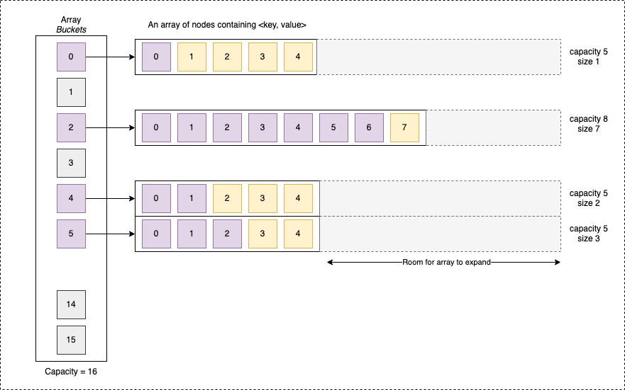
Separate Chaining (Dynamically growing array buckets)
The previous implementation, while functional, is a bit naive. In a production environment, the “Separate Chaining with Linked Lists” approach has a significant “elephant in the room”: Cache Unfriendliness.
Modern CPUs are designed to be incredibly fast, but they are often bottlenecked by the speed of RAM. To solve this, CPUs use a hierarchy of caches. They are optimized to predict memory access patterns, specifically looking for two things: recently accessed memory and contiguous memory (spatial locality).
In a linked list, nodes are scattered across the heap depending on where malloc() finds space. When you call node->next, the CPU often has to wait for a “cache miss” because the next node isn’t in the cache. This makes iteration and reading quite slow on modern hardware.
By switching to a “self-expanding” array, something akin to C++’s std::vector or Java’s ArrayList, we ensure that all colliding elements in a bucket are stored in contiguous memory.
The Trade-off:
- Pros: Drastically reduced cache misses during lookups.
- Cons: Resizing the bucket array via
realloc(or a manual copy) is expensive, meaning “writes” become significantly more costly when the array needs to grow.
Visually, our new hash table structure looks like this:
Writing a vector-like structure for our buckets: ch_vect
The model
To maintain our generic approach, we’ll use an array of void*. This allows each bucket to hold pointers to any data type.
#define VECT_INIT_CAPACITY (1<<2) // Start with 4 slots
#define VECT_GROWTH_MULTI (2)     // Double size on growth

typedef struct ch_vect_s {
    size_t capacity; // Total allocated slots
    size_t size;     // Actual elements currently stored
    void **array;    // The contiguous block of pointers
} ch_vect;
The interface
For our hash table’s needs, we only need a few core operations:
ch_vect* ch_vect_new(size_t capacity);
ch_vect* ch_vect_new_default();
void ch_vect_free(ch_vect *vect);
void* ch_vect_get(ch_vect *vect, size_t idx);
void ch_vect_set(ch_vect *vect, size_t idx, void *data);
void ch_vect_append(ch_vect *vect, void *data);
Memory Management
The allocation and de-allocation are standard, but we must be careful with our pointers:
ch_vect* ch_vect_new(size_t capacity) {
    ch_vect *result = malloc(sizeof(*result));
    if (NULL == result) exit(EXIT_FAILURE); // Reminder: exit() is bad for libs!

    result->capacity = capacity;
    result->size = 0;
    result->array = malloc(result->capacity * sizeof(*(result->array)));

    if (NULL == result->array) {
        free(result);
        exit(EXIT_FAILURE);
    }
    return result;
}

void ch_vect_free(ch_vect *vect) {
    free(vect->array);
    free(vect);
}
Appending and Growing
When the vector is full, we must expand it. We check for SIZE_MAX overflows before allocating a new, larger array and copying the old pointers over.
void ch_vect_append(ch_vect *vect, void *data) {
    if (vect->size >= vect->capacity) {
        // Growth logic
        size_t new_capacity = vect->capacity * VECT_GROWTH_MULTI;
        void **new_array = realloc(vect->array, new_capacity * sizeof(void*));

        if (NULL == new_array) exit(EXIT_FAILURE);

        vect->array = new_array;
        vect->capacity = new_capacity;
    }
    vect->array[vect->size++] = data;
}
Updating ch_hash to ch_hashv
To integrate this, we create ch_hashv. The primary difference is simply the type of the bucket array:
typedef struct ch_hashv_s {
    size_t capacity;
    size_t size;
    ch_vect **buckets; // Array of vector pointers instead of node pointers
    ch_key_ops key_ops;
    ch_val_ops val_ops;
} ch_hashv;
The logic remains mostly the same, but we swap the while loops (for linked lists) with for loops (for vectors). You can find the full implementation details on GitHub.
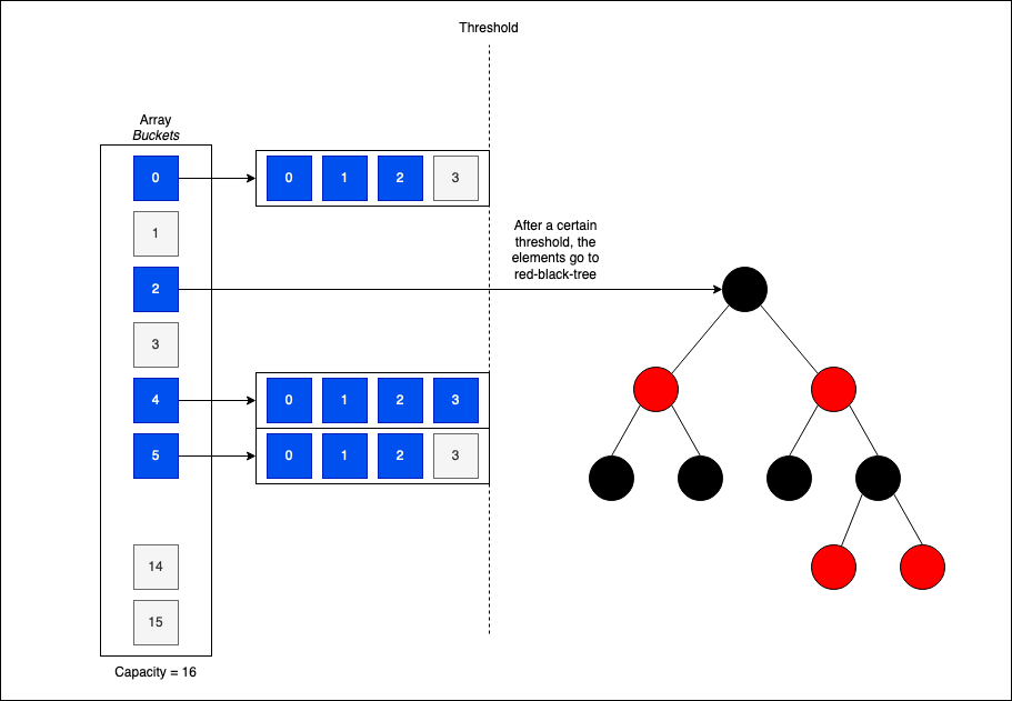
Separate Chaining (Red-Black Trees Optimization)
While ch_hashv improves read times via better cache locality, the theoretical search time in a bucket is still $O(N)$ if many collisions occur. To truly harden the data structure against worst-case scenarios, we can introduce Treeification.
If the number of colliding elements in a bucket exceeds a specific threshold (e.g., 8 elements), we can “morph” that bucket from a list or vector into a Red-Black Tree.
Red-Black trees are self-balancing binary search trees. This ensures that even with a high number of collisions, search performance stays within $O(\log N)$ bounds. This is exactly how the Java HashMap has operated since Java 8.
Open Addressing
Compared to Separate Chaining, a hash table implemented with Open Addressing stores exactly one element per bucket. There are no linked lists or vectors attached to the slots; instead, we handle collisions by searching for the next available unused slot directly within the main bucket array.
Finding these unused locations is achieved through a probing algorithm. This algorithm determines the sequence of indices to check (the 2nd, 3rd, or $n^{th}$ “natural” index) if the initial target bucket is already occupied.
Linear Probing
The most straightforward probing method is linear probing. If a collision occurs at bucket $i$, we simply check $i+1, i+2, \dots$ until we find an empty slot.
To prevent excessive probing, we must maintain a healthy load factor ($size/capacity$) and use a hash function with excellent diffusion. If the load factor reaches a certain threshold (often 0.7 or 0.8), we must expand the array and perform a full rehashing to redistribute the elements.
If we fail to keep the load factor low, clustering occurs.
The Problem of Clustering
Clustering significantly degrades performance for both reads and inserts because the CPU must iterate through long “blocks” of occupied slots to find a value or an empty space.
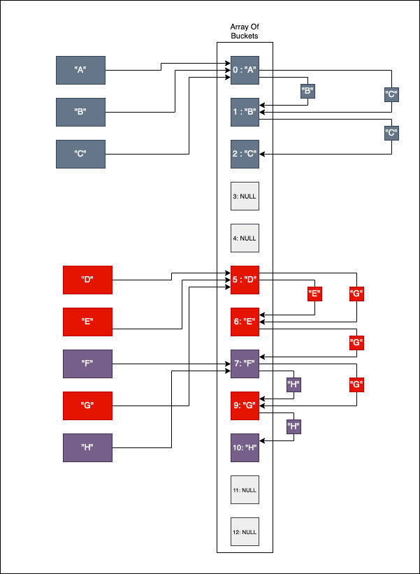
Consider the following example where we insert keys A through H:
- Insert “A”: Target bucket is
0. It’s free, so “A” settles there. - Insert “B”: Target bucket is
0. Occupied! We probe to index1, find it’s free, and insert “B”. - Insert “C”: Target bucket is
0. Occupied! We probe1(occupied), then2. “C” is inserted at2.
As we continue with "D" through "H", we create a dense “clump” of elements. This is a cluster. To read the value for "G", the algorithm might start at its natural hash position but then be forced to step through multiple unrelated entries before finding the correct one.
Clustering typically stems from two issues:
- High Load Factor: The array is too full, reducing the “breathing room” between entries.
- Poor Diffusion: The hash function is biased, consistently targeting the same narrow range of indices.
Beyond Linear Probing
To mitigate clustering, we can swap linear probing for more sophisticated algorithms:
- Quadratic Probing: Instead of stepping by 1, we use a quadratic function (e.g., $i + 1^2, i + 2^2, i + 3^2$) to “jump” further away from the initial collision, breaking up potential clusters.
- Double Hashing: We use a second hash function to determine the step size for probing. This ensures that two keys colliding at the same initial index will likely follow different probe sequences.
Why use Open Addressing?
While it is more complex to implement (especially deletion, which requires marking slots as “deleted” or “tombstones”), Open Addressing is incredibly cache-friendly. Since all data resides in a single contiguous block of memory, the CPU can pre-fetch data far more effectively than it can when chasing linked list pointers.
Languages like Python (for its dict implementation) and Rust use advanced variants of Open Addressing precisely because of this superior raw performance on modern hardware.
Tombstones
Deleting elements in an Open Addressing hash table is significantly more challenging than in Separate Chaining. In a chained table, you simply snip a node out of a linked list. In Open Addressing, you can’t just set a bucket to NULL and call it a day.
If you simply empty a bucket, you break the “probe chain.” Any elements that were pushed further down the array due to a collision with the now-deleted item become mathematically unreachable. The search algorithm will hit that new NULL slot, assume the key doesn’t exist, and stop, even though the data is sitting right in the next slot.
One naive solution is to rehash the entire table after every deletion. However, allocating a new array and re-calculating every index is a massive performance tax that no one wants to pay.
The Sentinel Solution
The standard alternative is to use Tombstones. When an entry is deleted, instead of clearing the slot, we replace it with a sentinel value, a “tombstone.”
The tombstone changes its behavior based on what you are trying to do:
- For
GETorDELETEoperations: The tombstone acts as a “keep going” sign. The probing algorithm sees the tombstone, ignores it, and continues to the next slot. This ensures the rest of the probe sequence remains intact.
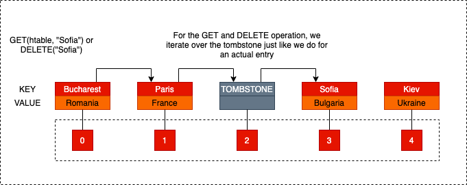
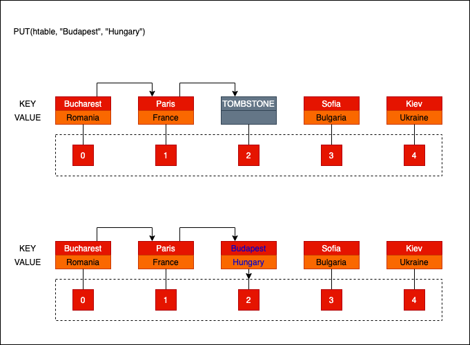
- For
PUT(Insert) operations: The tombstone acts as an inviting empty slot. If we find a tombstone during an insertion, we can reclaim that space and bury the new data there.
Managing Tombstone Density
There is a catch: tombstones don’t reduce the load factor. If your table becomes 20% data and 60% tombstones, your search performance will feel like an 80% full table because you are constantly probing through “dead” slots. An intelligent implementation must eventually trigger a rehash to clear out the “graveyard” when the tombstone density gets too high.
While there are clever ways to avoid tombstones by shifting elements back to fill gaps, they are significantly more complex. For our implementation, we will stick to the tombstone method, it’s the classic, academic approach to the problem.
A Generic Implementation
If you want to jump directly into the code without reading the full explanation, you can clone the repository here:
git clone git@github.com:nomemory/open-adressing-hash-table-c.git
Consistent with our Separate Chaining implementation, we will use void* pointers to achieve genericity, allowing the table to store any data type while keeping the core logic decoupled from the specific data formats.
The Model
The model layer for Open Addressing remains familiar, but with a few key adjustments to accommodate how data is laid out in memory.
First, we define our “traits” for keys and values. These allow the table to hash, copy, compare, and free data it doesn’t natively understand.
typedef struct oa_key_ops_s {
    uint32_t (*hash)(const void *data, void *arg);
    void* (*cp)(const void *data, void *arg);
    void (*free)(void *data, void *arg);
    bool (*eq)(const void *data1, const void *data2, void *arg);
    void *arg;
} oa_key_ops;

typedef struct oa_val_ops_s {
    void* (*cp)(const void *data, void *arg);
    void (*free)(void *data, void *arg);
    bool (*eq)(const void *data1, const void *data2, void *arg);
    void *arg;
} oa_val_ops;
Next, we define the oa_pair, which represents the actual <key, value> entry stored in the table. We include the hash here so we don’t have to recompute it during rehashing.
typedef struct oa_pair_s {
    uint32_t hash;
    void *key;
    void *val;
} oa_pair;
Finally, the main oa_hash structure manages the collection:
typedef struct oa_hash_s {
    size_t capacity;     // Total number of buckets
    size_t size;         // Number of active elements
    oa_pair **buckets;   // Contiguous array of pair pointers
    void (*probing_fct)(struct oa_hash_s *htable, size_t *idx); // Probing strategy
    oa_key_ops key_ops;  // Key-specific operations
    oa_val_ops val_ops;  // Value-specific operations
} oa_hash;
Key features of this structure:
buckets: Unlike Separate Chaining, where buckets lead to lists, here each bucket holds a direct reference to a singleoa_pair.probing_fct: This is a function pointer that defines our collision resolution strategy. By making this swappable, we can easily switch between different algorithms.
Probing Strategies
For Linear Probing, we implement a simple function that increments the index. If it hits the end of the array, it wraps back around to the start (circular buffer logic).
static inline void oa_hash_lp_idx(oa_hash *htable, size_t *idx) {
    (*idx)++;
    if ((*idx) == htable->capacity) {
        (*idx) = 0; // Wrap around
    }
}
This flexibility allows us to implement Quadratic Probing or other strategies later without rewriting the core GET and PUT logic.
Configuration Constants
To ensure the table remains performant and doesn’t suffer from excessive clustering, we define the following thresholds:
#define OA_HASH_LOAD_FACTOR (0.75)   // Resize when 75% full
#define OA_HASH_GROWTH_FACTOR (1<<2) // 4x growth on resize
#define OA_HASH_INIT_CAPACITY (1<<12) // Initial capacity of 4096
OA_HASH_LOAD_FACTOR: In Open Addressing, performance drops sharply as the table fills up. 0.75 is a common industry standard to balance memory usage and speed.OA_HASH_GROWTH_FACTOR: We use a significant growth factor to reduce the frequency of expensive rehashing operations.OA_HASH_INIT_CAPACITY: A reasonably large starting size to minimize early-stage rehashes.
The interface
The interface is again relatively straightforward:
// Creating  anew hash table
oa_hash* oa_hash_new(oa_key_ops key_ops, oa_val_ops val_ops, void (*probing_fct)(struct oa_hash_s *htable, size_t *from_idx));
oa_hash* oa_hash_new_lp(oa_key_ops key_ops, oa_val_ops val_ops);
// Destructor like method for destroying the hashtable
void oa_hash_free(oa_hash *htable);
// Adding, Reading, Deleting entries
void oa_hash_put(oa_hash *htable, const void *key, const void *val);
void *oa_hash_get(oa_hash *htable, const void *key);
void oa_hash_delete(oa_hash *htable, const void *key);
void oa_hash_print(oa_hash *htable, void (*print_key)(const void *k), void (*print_val)(const void *v));

// Pair related
oa_pair *oa_pair_new(uint32_t hash, const void *key, const void *val);

// String operations
uint32_t oa_string_hash(const void *data, void *arg);
void* oa_string_cp(const void *data, void *arg);
bool oa_string_eq(const void *data1, const void *data2, void *arg);
void oa_string_free(void *data, void *arg);
void oa_string_print(const void *data);
Creating/Destroying a hash table
As with any complex data structure in C, we start by defining our constructor-like and destructor-like functions to manage the lifecycle of the oa_hash structure on the heap.
oa_hash_new: Dynamically allocates the table and initializes its metadata and bucket array.oa_hash_free: Performs a deep cleanup, ensuring every pair and its generic data are properly deallocated to prevent memory leaks.
oa_hash* oa_hash_new(
    oa_key_ops key_ops,
    oa_val_ops val_ops,
    void (*probing_fct)(struct oa_hash_s *htable, size_t *idx))
{
    oa_hash *htable = malloc(sizeof(*htable));
    if (NULL == htable) {
        fprintf(stderr, "malloc() failed in file %s at line # %d\n", __FILE__, __LINE__);
        exit(EXIT_FAILURE);
    }

    htable->size = 0;
    htable->capacity = OA_HASH_INIT_CAPACITY;
    htable->val_ops = val_ops;
    htable->key_ops = key_ops;
    htable->probing_fct = probing_fct;

    // Allocate the contiguous array of bucket pointers
    htable->buckets = malloc(sizeof(*(htable->buckets)) * htable->capacity);
    if (NULL == htable->buckets) {
        free(htable);
        exit(EXIT_FAILURE);
    }

    // Initialize all buckets to NULL (empty)
    for(size_t i = 0; i < htable->capacity; i++) {
        htable->buckets[i] = NULL;
    }

    return htable;
}
To simplify things for the user, we can provide a specialized allocator that defaults to linear probing:
oa_hash* oa_hash_new_lp(oa_key_ops key_ops, oa_val_ops val_ops) {
    return oa_hash_new(key_ops, val_ops, oa_hash_lp_idx);
}
The destructor, oa_hash_free, must traverse the entire bucket array. For every non-null slot, it uses the provided free traits to clean up the generic key and value before freeing the oa_pair container itself.
void oa_hash_free(oa_hash *htable) {
    for(size_t i = 0; i < htable->capacity; i++) {
        if (NULL != htable->buckets[i]) {
            // Only free key/val if it's an actual entry (not a tombstone)
            if (htable->buckets[i]->key)
                htable->key_ops.free(htable->buckets[i]->key, htable->key_ops.arg);
            if (htable->buckets[i]->val)
                htable->val_ops.free(htable->buckets[i]->val, htable->val_ops.arg);

            free(htable->buckets[i]);
        }
    }
    free(htable->buckets);
    free(htable);
}
Modeling Tombstones
To implement deletion correctly in Open Addressing, we need to represent tombstones. A tombstone is a “zombie” entry: the slot is technically occupied, but it contains no data. We define a tombstone as a non-NULL oa_pair where the key and val are NULL and the hash is 0.
We use a helper function to identify these sentinel values during our probing sequences:
inline static bool oa_hash_is_tombstone(oa_hash *htable, size_t idx) {
    oa_pair *p = htable->buckets[idx];
    // A tombstone is a bucket that is not NULL but has NULL data
    return (p != NULL && p->key == NULL && p->val == NULL);
}
And a corresponding function to “bury” an entry by turning it into a tombstone when a deletion occurs:
inline static void oa_hash_put_tombstone(oa_hash *htable, size_t idx) {
    if (NULL != htable->buckets[idx]) {
        // Free existing data first to avoid leaks!
        htable->key_ops.free(htable->buckets[idx]->key, htable->key_ops.arg);
        htable->val_ops.free(htable->buckets[idx]->val, htable->val_ops.arg);

        // Mark as tombstone
        htable->buckets[idx]->hash = 0;
        htable->buckets[idx]->key = NULL;
        htable->buckets[idx]->val = NULL;
    }
}
Growing the bucket capacity if needed
To maintain high performance in an Open Addressing hash table, we must monitor the Load Factor ($\alpha = \frac{\text{size}}{\text{capacity}}$). As the table fills up, the probability of collisions increases exponentially, leading to longer probe sequences. A common industry standard is to grow the table once the load factor exceeds 0.75.
We define a helper function, oa_hash_should_grow, to perform this check after every insertion:
#define OA_HASH_LOAD_FACTOR (0.75)

inline static bool oa_hash_should_grow(oa_hash *htable) {
    // Note: Cast to float or use multiplication to avoid integer division issues
    return (double)htable->size / htable->capacity > OA_HASH_LOAD_FACTOR;
}
If the threshold is hit, we call oa_hash_grow. This method handles the complex task of expanding the table while keeping the data intact:
- Capacity Overflow Check: Ensures we don’t exceed the architectural limits of
size_t. - Allocation: Reserves a new, larger memory block for the buckets.
- Rehashing: Iterates through the old buckets and re-inserts every valid entry into the new array. Crucially, tombstones are skipped during this process, effectively “cleaning” the graveyard.
- Cleanup: Frees the old bucket array.
inline static void oa_hash_grow(oa_hash *htable) {
    uint32_t old_capacity;
    oa_pair **old_buckets;

    // 1. Check if the new capacity overflows SIZE_MAX
    uint64_t new_capacity_64 = (uint64_t) htable->capacity * OA_HASH_GROWTH_FACTOR;
    if (new_capacity_64 > SIZE_MAX) {
        fprintf(stderr, "Size overflow in %s at line %d\n", __FILE__, __LINE__);
        exit(EXIT_FAILURE);
    }

    old_capacity = htable->capacity;
    old_buckets = htable->buckets;

    // 2. Setup the expanded table
    htable->capacity = (uint32_t) new_capacity_64;
    htable->size = 0; // Reset size as oa_hash_put will increment it
    htable->buckets = malloc(htable->capacity * sizeof(*(htable->buckets)));

    if (NULL == htable->buckets) {
        fprintf(stderr, "malloc() failed\n");
        exit(EXIT_FAILURE);
    }

    for(size_t i = 0; i < htable->capacity; i++) {
        htable->buckets[i] = NULL;
    }

    // 3. Rehash elements (skipping tombstones)
    for(size_t i = 0; i < old_capacity; i++) {
        oa_pair *crt_pair = old_buckets[i];

        // Only re-insert actual entries, effectively purging tombstones
        if (crt_pair != NULL && !oa_hash_is_tombstone(htable, i)) {
            oa_hash_put(htable, crt_pair->key, crt_pair->val);

            // Clean up the old pair container (data is copied into the new table)
            htable->key_ops.free(crt_pair->key, htable->key_ops.arg);
            htable->val_ops.free(crt_pair->val, htable->val_ops.arg);
            free(crt_pair);
        } else if (crt_pair != NULL) {
            // It's a tombstone; just free the container
            free(crt_pair);
        }
    }

    // 4. Final cleanup
    free(old_buckets);
}
Finding the Right Bucket Index
In Open Addressing, we need a robust way to locate the correct index for three main operations: GET, PUT, and DELETE. This logic is centralized in the helper function oa_hash_getidx.
The challenge is that the target index behaves differently depending on the operation. When we PUT data, we want to find either the original key (to update it) or the first available “hole” (which includes both NULL slots and tombstones). However, when we GET or DELETE, we must treat tombstones as “occupied” slots to ensure we don’t break the probe chain and skip over keys pushed further down the array.
static size_t oa_hash_getidx(oa_hash *htable, size_t idx, uint32_t hash_val, const void *key, enum oa_ret_ops op) {
    do {
        // Condition 1: If we are inserting (PUT), we can reclaim a tombstone slot.
        if (op == PUT && oa_hash_is_tombstone(htable, idx)) {
            break;
        }

        // Condition 2: Check if the current bucket contains our key.
        // We compare the integer hash first for speed before calling the equality trait.
        if (htable->buckets[idx] != NULL && !oa_hash_is_tombstone(htable, idx)) {
            if (htable->buckets[idx]->hash == hash_val &&
                htable->key_ops.eq(key, htable->buckets[idx]->key, htable->key_ops.arg)) {
                break;
            }
        }

        // Collision: Use the probing function pointer to find the next candidate index.
        htable->probing_fct(htable, &idx);

    } while(NULL != htable->buckets[idx]);

    return idx;
}
The logic flow for idx (the starting point) is always the “natural” bucket:
uint32_t hash_val = htable->key_ops.hash(key, htable->key_ops.arg);
size_t idx = hash_val % htable->capacity;
If the natural bucket is occupied by a different key, oa_hash_getidx will cycle through the probe sequence (linearly or quadratically) until it finds a match, a recyclable tombstone (only for PUT), or an empty NULL slot.
Adding an Element to the Hash Table
The oa_hash_put method manages the insertion and update logic. It ensures the table remains efficient by triggering a growth phase if the load factor gets too high, then finds the best available slot for the new data.
The steps for oa_hash_put are:
- Scale if necessary: Check if the table needs to grow before adding new data.
- Locate the index: Find the natural bucket or the next available slot via probing.
- Update or Insert: If the index contains the same key, update the value. Otherwise, allocate a new pair and “bury” it in the empty slot or tombstone.
void oa_hash_put(oa_hash *htable, const void *key, const void *val) {
    // 1. Maintain a healthy load factor
    if (oa_hash_should_grow(htable)) {
        oa_hash_grow(htable);
    }

    uint32_t hash_val = htable->key_ops.hash(key, htable->key_ops.arg);
    size_t idx = hash_val % htable->capacity;

    // 2. Optimization: If the natural bucket is NULL, insert immediately.
    // Otherwise, use the probing logic to find the correct index.
    if (NULL != htable->buckets[idx]) {
        idx = oa_hash_getidx(htable, idx, hash_val, key, PUT);
    }

    if (NULL == htable->buckets[idx] || oa_hash_is_tombstone(htable, idx)) {
        // 3a. Key doesn't exist or we found a tombstone: Create a new entry.
        // If it's a tombstone, we free the old "empty" container first.
        if (htable->buckets[idx]) free(htable->buckets[idx]);

        htable->buckets[idx] = oa_pair_new(
                hash_val,
                htable->key_ops.cp(key, htable->key_ops.arg),
                htable->val_ops.cp(val, htable->val_ops.arg)
        );
        htable->size++;
    } else {
        // 3b. Key already exists: Update the entry.
        // Clean up old data via traits before assigning new copies.
        htable->val_ops.free(htable->buckets[idx]->val, htable->val_ops.arg);
        htable->key_ops.free(htable->buckets[idx]->key, htable->key_ops.arg);

        htable->buckets[idx]->val = htable->val_ops.cp(val, htable->val_ops.arg);
        htable->buckets[idx]->key = htable->key_ops.cp(key, htable->key_ops.arg);
        htable->buckets[idx]->hash = hash_val;
    }
}
By allowing PUT to “stop” at tombstones, we effectively recycle the memory graveyard, keeping our probe chains as short as possible without needing a full rehash.
Removing an element from the hash table
Deleting an entry in Open Addressing isn’t as simple as clearing a bucket. To keep our probe chains intact, we use the logic of tombstones.
The process for oa_hash_delete is as follows:
- Direct Check: We look at the “natural” bucket. If it’s empty (
NULL), the key isn’t there, so we exit. - Probing: If the natural bucket is occupied but doesn’t match our key, we use
oa_hash_getidxwith theDELETEflag. This ensures we jump over tombstones to find the actual data. - Cleanup & Burial: Once found, we free the memory for the key and value using our data traits, then we place a tombstone sentinel in that slot.
void oa_hash_delete(oa_hash *htable, const void *key) {
    uint32_t hash_val = htable->key_ops.hash(key, htable->key_ops.arg);
    size_t idx = hash_val % htable->capacity;

    // If the starting bucket is empty, there's nothing to delete
    if (NULL == htable->buckets[idx]) {
        return;
    }

    // Find the actual index of the key
    idx = oa_hash_getidx(htable, idx, hash_val, key, DELETE);

    // If the key wasn't found in the probe chain
    if (NULL == htable->buckets[idx] || oa_hash_is_tombstone(htable, idx)) {
        return;
    }

    // Free user data
    htable->val_ops.free(htable->buckets[idx]->val, htable->val_ops.arg);
    htable->key_ops.free(htable->buckets[idx]->key, htable->key_ops.arg);

    // Place the sentinel tombstone
    oa_hash_put_tombstone(htable, idx);
    htable->size--;
}
Retrieving an element from the hash table
Retrieving data follows the same probing logic. We must continue searching until we either find the matching key or hit a truly empty (NULL) slot. Tombstones are treated as “occupied” during the search to ensure we don’t stop prematurely.
void *oa_hash_get(oa_hash *htable, const void *key) {
    uint32_t hash_val = htable->key_ops.hash(key, htable->key_ops.arg);
    size_t idx = hash_val % htable->capacity;

    // If the natural bucket is empty, the key definitely isn't here
    if (NULL == htable->buckets[idx]) {
        return NULL;
    }

    // Locate the index using the GET operation logic
    idx = oa_hash_getidx(htable, idx, hash_val, key, GET);

    // If we hit a NULL or a tombstone, the key doesn't exist
    if (NULL == htable->buckets[idx] || oa_hash_is_tombstone(htable, idx)) {
        return NULL;
    }

    return htable->buckets[idx]->val;
}
Putting it all together
Using our generic Open Addressing table is now quite simple. Here’s a quick test using the string traits we defined earlier:
int main(int argc, char *argv[]) {
    // Create the table using linear probing
    oa_hash *h = oa_hash_new(oa_key_ops_string, oa_val_ops_string, oa_hash_lp_idx);

    // Insert entries
    oa_hash_put(h, "Bucharest", "Romania");
    oa_hash_put(h, "Sofia", "Bulgaria");

    // Fetch and print
    printf("Capital: Bucharest | Country: %s\n", (char*)oa_hash_get(h, "Bucharest"));
    printf("Capital: Sofia     | Country: %s\n", (char*)oa_hash_get(h, "Sofia"));

    // Cleanup
    oa_hash_free(h);

    return 0;
}
If you want to see how these concepts translate to other languages, feel free to check out my post on Java Hash Tables. The syntax is different, but the fundamental logic (probing, load factors, and collisions) remains universal.
References
- Hash Functions and Hash Tables, Breno Helfstein Moura
- Crafting Interpreters - Hash Tables, Robert Nystrom
- Hash functions
- CS240 – Lecture Notes: Hashing
- Hash Functions: An Empirical Comparison
- CSci 335 Software Design and Analysis - Chapter 5 Hashing and Hash Tables, Steward Weiss
- CSE 241 Algorithms and Data Structures - Chosing hash functions
- Integer hash functions, Thomas Wang
- Notes on Data Structures and Programming Techniques, James Aspnes
- The FNV Non-Cryptographic Hash Algorithm
- Hash Tables - Open Addressing vs Chaining;
- Optimizing software in C++, Agner Fog
- Why did the designers of Java preferred chaining over open addressing
- Deletion from hash tables without tombstones
- Traits
Source Code & Contributions
Spot an error or have an improvement? Open a PR directly for this article .