Introduction

There are rumors saying Computer Vision Engineers consider Eigenvalues and Eigenvectors the single most important concept(s) in linear algebra. I am not 100% sure about that, but I must admit those two things confused me a lot during my university years.

I think my teacher lost me somewhere in between The basis of a vector space and Linear transformations. N-dimensional vectors rotating?! That was too much for me. So I stopped caring, learned the formulas, and passed the exam. Here I am more than ten years later, interested in A.I. algorithms and realizing those two notions are much simpler than I thought.

But, before jumping directly into the subject, we must first talk about a few auxiliary concepts that will help us better understand the mystery behind Eigenvectors and Eigenvalues.

Think of matrices as functions

In mathematics, a function is a rule that accepts an input and produces an output.

For example, $f(x) = x + 1$ where $f : \mathbb{N} \rightarrow \mathbb{N}$ is a function that accepts a natural number $x$, increments it by $1$, and returns the result. As expected, $f(0) = 0 + 1 = 1$ and $f(5) = 5 + 1 = 6$. If $x$ varies, the result varies.

Now let’s think of a matrix $A$ with $m$ rows and $n$ columns ($A \in \mathbb{R}^{m \times n}$). Consider the equation $b = A x$ where:

• $x$ is an n-dimensional vector, $x \in \mathbb{R}^n$
• $b$ is an m-dimensional vector, $b \in \mathbb{R}^m$

If we change $x$, $b$ will likely change. In this sense, $A$ acts exactly like a function: it takes a vector from one space and maps it to another.

Forcing the mathematical notation a little, we can say: $A(x) = b \text{, where } A : \mathbb{R}^n \rightarrow \mathbb{R}^m$.

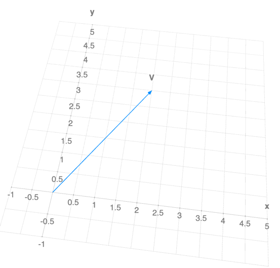
Example 1:

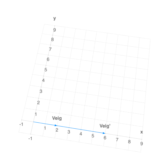
Consider a bi-dimensional vector:

If we were to plot this vector in the 2D plane, it would look like this:

Now, let’s define a matrix $A = \begin{bmatrix} 1 & 0 \ 0 & 0 \end{bmatrix}$ and compute $A V$:

By applying the “matrix” function to our vector, $A(V)=V^{’}$, we removed the $y$ component. If we plot it:

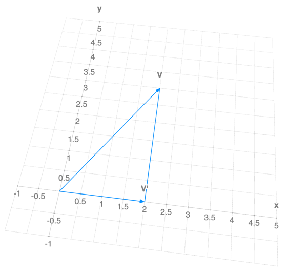
We can observe that $V^{’}$ is the projection of $V$ onto the x-axis. Thus, matrix $A$ works as a function that projects any vector to the x-axis.

Matrix transformations

A transformation $T$ is a “rule” that assigns to each vector $v \in \mathbb{R}^n$ a vector $T(v) \in \mathbb{R}^m$.

• $T(x) \in \mathbb{R}^m$ is the image of $x \in \mathbb{R}^n$ under $T$;
• All images $T(x)$ constitute the range of $T$;
• $\mathbb{R}^n$ is the domain of $T$;
• $\mathbb{R}^m$ is the co-domain of $T$;

Let $A$ be an $m \times n$ matrix. The matrix transformation associated with $A$ is defined by: $T(x) = A x$.

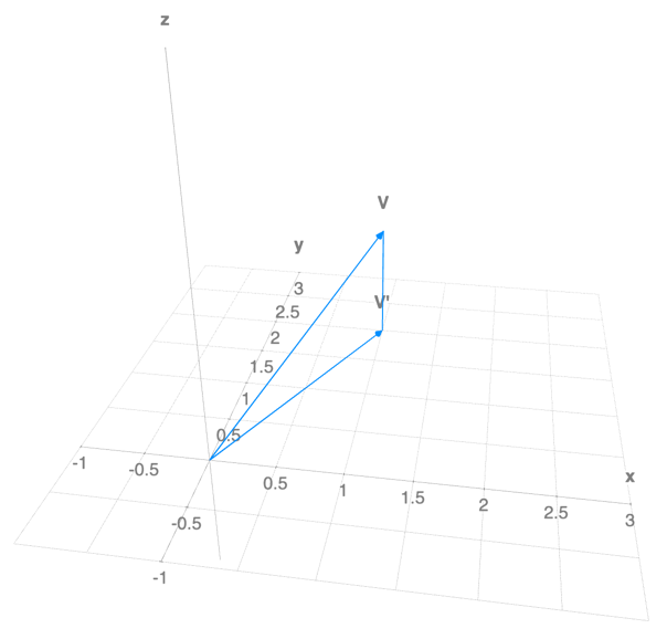
Example: Projection on the (x, y) plane

Let $A$ be:

If we form the matrix transformation equation $A v = b$:

The $z$ information has “evaporated.” The matrix $A$ projected our 3D vector $v$ onto the 2D xy-plane.

Linear Transformations

A linear transformation is a Transformation $T:\mathbb{R}^n \rightarrow \mathbb{R}^m$ satisfying:

where $u, v \in \mathbb{R}^n$ and $c$ is a scalar. In matrix notation:

• Linear transformations always map the zero vector to the zero vector: $T(0) = 0$.
• For any combination of vectors and scalars: $T(c_{1} v_{1} + \dots + c_{k} v_{k}) = c_{1} T(v_{1}) + \dots + c_{k} T(v_{k})$.

Note that a “translation” like:

is not linear, because $T(0) = \begin{bmatrix} 1 \ 2 \ 3 \end{bmatrix} \neq 0$.

Key takeaway: Every linear transformation is a matrix transformation!

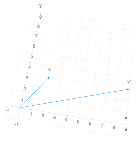
For example, the matrix

describes a linear transformation.

If we apply it to

We obtain:

The vector was “stretched” and its orientation changed.

Eigenvalues and Eigenvectors

For a square transformation matrix $A \in \mathbb{R}^{n \times n}$:

• An eigenvector is a non-zero vector $v$ such that $A v = \lambda v$ for some scalar $\lambda$.
• An eigenvalue is the scalar $\lambda$ that makes this equation possible for a non-trivial $v$.

In simple terms, an eigenvector is a special vector that does not change its direction (it stays on its original span) when the transformation is applied; it only gets scaled (stretched or shrunk) by the eigenvalue $\lambda$.

To compute them, we rearrange the equation:

For example, if:

Then we solve the characteristic equation:

We find $\lambda_{1}=3, \lambda_{2}=1$. Plugging $\lambda$ back into $(A - \lambda I)v = 0$ gives the vectors:

• For $\lambda_{1} = 1$, an eigenvector is $v_{1} = \begin{bmatrix} -1 \ 2 \end{bmatrix}$.
• For $\lambda_{2} = 3$, an eigenvector is $v_{2} = \begin{bmatrix} 1 \ 0 \end{bmatrix}$.

Observation: For a triangular matrix, the eigenvalues are simply the elements on the main diagonal!

Why are they “special”?

If we transform a “normal” vector

with our matrix $A$, it rotates and stretches, landing off its original line of action:

But if we transform an eigenvector

then

The vector stays on the same line (same span)! It just got 3 times longer.

Why are they important?

In Computer Engineering and Data Science, these concepts are the bedrock of:

• Principal Component Analysis (PCA): Reducing data dimensions by finding the axes (eigenvectors) along which the data varies the most.
• Image Compression: Keeping only the most “important” eigenvalues to reconstruct an image with less data.
• PageRank: Google’s algorithm treats the web as a giant matrix where the most important pages are found using an eigenvector.
• Vibration Analysis: Engineers use them to find the “natural frequencies” of structures like bridges so they don’t collapse.

Where to go next

If you want to find out how to compute Eigenvectors and Eigenvalues programmatically, check out my next article.